-

Want a paper copy?
You can now buy the book!
All royalties go to the Cystic Fibrosis Trust.Spotted an error? Have comments?
Let us know!Get hands on with source code for the book.
2.2 Testing out the model
Having constructed a model, the first thing to do is to test it out with some simple example data to check that its behaviour is reasonable. Suppose a candidate knows C# but not SQL – we would expect them to get the first question right and the other two questions wrong. So let’s test the model out for this case and see what skills it infers for that pattern of answers. For convenience, we’ll use isCorrect to refer to the array [isCorrect1,isCorrect2,isCorrect3] and so we will consider the case where isCorrect is [true,false,false].
We want to infer the probability that the candidate has the csharp and sql skills, given this particular set of isCorrect values. This is an example of an inference query which is defined by the variables we want to infer (csharp, sql) and the variables we are conditioning on (isCorrect) along with their observed values. Because this example is quite small, we can work out the answer to this inference query by hand.
Doing inference by hand
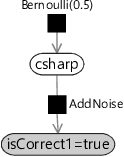
To get started, let’s look at how to infer the probability for the csharp skill given the answer to just the first question. Dropping other variables gives the simplified factor graph shown in Figure 2.6.
|
This factor graph now looks just like the one for the murder mystery in section 1.3 and, just like for the murder mystery, we can apply Bayes’ theorem to solve it:
In equation (2.5) we have colour coded some of the terms to help track them through the calculation. Putting in numbers for csharp being true and false gives:
These numbers sum to 0.55. To get probabilities, we need to scale both numbers to sum to 1 (by dividing by 0.55) which gives:
So, given just the answer to the first question, the probability of having the csharp skill is .
Performing inference manually for all three questions is a more involved calculation. If you want to explore this calculation please read the following deep dive section. If not, skip over it to see how we can automate this inference calculation.
In this optional section, we perform inference manually in our three-question model by marginalising the joint distribution. Feel free to skip this section.
As we saw in Chapter 1, we can perform inference by marginalising the joint distribution (summing it over all the variables except the one we are interested in) while fixing the values of any observed variables. For the three-question factor graph, we wrote down the joint probability distribution in equation (2.4). Here it is again:
Before we start this inference calculation, we need to show how to compute a product of distributions. Suppose for some variable x, we know that:
This may look odd since we normally only associate one distribution with a variable but, as we’ll see, products of distributions arise frequently when performing inference. Evaluating this expression for the two values of x gives:
Since we know that and must add up to one, we can divide these values by to get:
This calculation may feel familiar to you – it is very similar to the inference calculations that we performed in Chapter 1.
In general, if want to multiply two Bernoulli distributions, we can use the rule that:
If, say, the second distribution is uniform (b=0.5), the result of the product is . In other words, the distribution is unchanged by multiplying by a uniform distribution. In general, multiplying any distribution by the uniform distribution leaves it unchanged.
Armed with the ability to multiply distributions, we can now compute the probability that our example candidate has the csharp skill. The precise probability we want to compute is , where we have abbreviated true to T and false to F. As before, we can compute this by marginalising the joint distribution and fixing the observed values:
As we saw in Chapter 1, we use the proportional sign because we do not care about the scaling of the right hand side, only the ratio of its value when csharp is true to the value when csharp is false.
Now we put in the full expression for the joint probability from (2.8) and fix the values of all the observed variables. We can ignore the Bernoulli(0.5) terms since, as we just learned, multiplying a distribution by a uniform distribution leaves it unchanged. So the right hand side of (2.13) becomes
Terms inside of each summation that do not mention the variable being summed over can be moved outside of the summation, because they have the same value for each term being summed. You can also think of this as moving the summation signs in towards the right:
If you look at the first term here, you’ll see that it is a function of csharp only, since isCorrect1 is observed to be true. When csharp is true, this term has the value 0.9. When csharp is false, this term has the value 0.2. Since we only care about the relative sizes of these two numbers, we can replace this term by a Bernoulli term where the probability of true is and the probability of false is therefore 1-0.818=0.182. Note that this has preserved the true/false ratio .
Similarly the second AddNoise term has value 0.1 when sql is true and the value 0.8 when sql is false, so can be replaced by a Bernoulli term where the probability of true is . The final AddNoise term can also be replaced, giving:
For the deterministic And factor, we need to consider the four cases where the factor is not zero (which we saw in Panel 2.1) and plug in the Bernoulli(0.111) distributions for sql and hasSkills in each case:
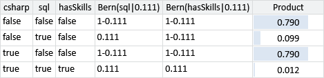
Looking at Table 2.3, we can see that when csharp is true, either both sql and hasSkills are false (with probability 0.790) or both sql and hasSkills are true (with probability 0.012). The sum of these is 0.802. When csharp is false, the corresponding sum is . So we can replace the last three terms by a Bernoulli term with parameter .
Now we have a product of Bernoulli distributions, so we can use (2.12) to multiply them together. When csharp is true, this product has value . When csharp is false, the value is . Therefore, the product of these two distributions is a Bernoulli whose parameter is :
So we have calculated that the posterior probability that our candidate has the csharp skill to be 80.2%. If we work through a similar calculation for the sql skill, we find the posterior probability is 3.4%. Together these probabilities say that the candidate is likely to know C# but is unlikely to know SQL, which seems like a very reasonable inference given that the candidate only got the C# question right.
Doing inference by passing messages on the graph
Doing inference calculations manually takes a long time and it is easy to make mistakes. Instead, we can do the same calculation mechanically by using a message passing algorithm. This works by passing messages along the edges of the factor graph, where a message is a probability distribution over the variable that the edge is connected to. We will see that using a message passing algorithm lets us do the inference calculations automatically – a huge advantage of the model-based approach!
To understand how message passing works, take another look at equation (2.6):
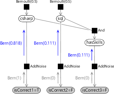
Figure 2.7 shows these colour-coded terms as messages being passed from one node to another node in the graph. For example, the factor node for the prior over csharp sends this prior distribution as a message to the csharp node (in blue). The observed isCorrect1 node sends an upwards message which is a point mass at the observed value (in red). The AddNoise factor transforms this message using Bayes’ theorem and outputs its own upwards message (in green). Each of these messages can be computed from information available at the node they are sent from.
Bernouilli(1.0)Bernoulli(0.5)Bernoulli(0.9/0.9+0.2)
|
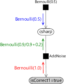
At this point the two messages arriving at the csharp node provide all the information we need to compute the posterior distribution for the csharp variable, as we saw in equation (2.6). This method of using message passing to compute posterior distributions is called belief propagation [Pearl, 1982; Pearl, 1988; Lauritzen and Spiegelhalter, 1988].
If you would like to see how to use belief propagation to compute posterior distributions in our three-question model, read the next section. Otherwise, you can skip straight to the results.
In this optional section, we show how belief propagation can be used to perform inference in our three-question model. Feel free to skip this section.
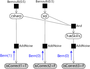
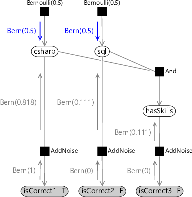
Let us redo the inference calculation for the csharp skill using message passing – we’ll describe the message passing process for this example first, and then look at the general form later on. The first step in the manual calculation was to fix the values of the observed variables. Using message passing, this corresponds to each observed variable sending out a message which is a point mass distribution at the observed value. In our case, each isCorrect variable sends the point mass Bernoulli(0) if it is observed to be false or the point mass Bernoulli(1) if it is observed to be true. This means that the three messages sent are as shown in Figure 2.8.
Bern(1)Bern(0)Bern(0)
|
These point mass messages then arrive at the AddNoise factor nodes. The outgoing messages at each factor node can be computed separately as follows:
- The message up from the first AddNoise factor to csharp can be computed by writing as a Bernoulli distribution over csharp. As we saw in the last section, the parameter of the Bernoulli is , so the upward message is .
- The message up from the second AddNoise factor to sql can be computed by writing as a Bernoulli distribution over sql. The parameter of the Bernoulli is , so the upward message is .
- The message up from the third AddNoise factor to hasSkills is the same as the second message, since it is computed for the same factor with the same incoming message. Hence, the third upward message is also .
Bern(1)Bern(0)Bern(0)Bern(0.818)Bern(0.111)Bern(0.111)
|
Note that these three messages are exactly the three Bernoulli distributions we saw in in (2.16). Rather than working on the entire joint distribution, we have broken down the calculation into simple, repeatable message computations at the nodes in the factor graph.
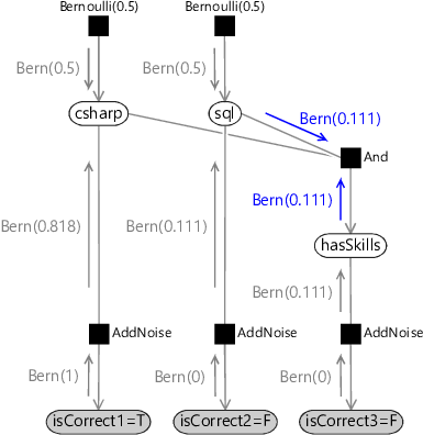
The messages down from the Bernoulli(0.5) prior factors are just the prior distributions themselves:
Bern(1)Bern(0)Bern(0)Bern(0.818)Bern(0.111)Bern(0.111)Bern(0.5)Bern(0.5)
|
The outgoing message for any variable node is the product of the incoming messages on the other edges connected to that node. For the sql variable node we now have incoming messages on two edges, which means we can compute the outgoing message towards the And factor. This is Bernoulli(0.111) since the upward message is unchanged by multiplying by the uniform downward message Bernoulli(0.5). The hasSkills variable node is even simpler: since there is only one incoming message, the outgoing message is just a copy of it.
Bern(1)Bern(0)Bern(0)Bern(0.5)Bern(0.818)Bern(0.5)Bern(0.111)Bern(0.111)Bern(0.111)Bern(0.111)
|
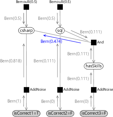
Finally, we can compute the outgoing message from the And factor to the csharp variable. This is computed by multiplying the incoming messages by the factor function and summing over all variables other than the one being sent to (so we sum over sql and hasSkills):
The summation gives the message Bernoulli(0.474), as we saw in equation (2.17).
Bern(1)Bern(0)Bern(0)Bern(0.5)Bern(0.818)Bern(0.5)Bern(0.111)Bern(0.111)Bern(0.111)Bern(0.111)Bern(0.474)
|
We now have all three incoming messages at the csharp variable node, which means we are ready to compute its posterior marginal. This is achieved by multiplying together the three messages – this is the calculation we performed in equation (2.17) and hence gives the same result Bernoulli(0.802) or 80.2%.
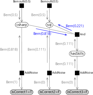
To compute the marginal for sql, we can re-use most of the messages we just calculated and so only need to compute two additional messages (shown in Figure 2.13). The first message, from csharp to the And factor, is the product of Bernoulli(0.818) and the uniform distribution Bernoulli(0.5), so the result is also Bernoulli(0.818).
The second message is from the And factor to sql. Again, we compute it by multiplying the incoming messages by the factor function and summing over all variables other than the one being sent to (so we sum over csharp and hasSkills):
The summation gives the message Bernoulli(0.221), so the two new messages we have computed are those shown in Figure 2.13.
Bern(1)Bern(0)Bern(0)Bern(0.5)Bern(0.818)Bern(0.5)Bern(0.111)Bern(0.111)Bern(0.111)Bern(0.818)Bern(0.221)
|
Multiplying this message into sql with the upward message from the AddNoise factor gives or 3.4%, the same result as before. Note that again we have ignored the uniform message from the prior, since multiplying by a uniform distribution has no effect.
The message passing procedure we just saw arises from applying the general belief propagation algorithm. In belief propagation, messages are computed in one of three ways, depending on whether the message is coming from a factor node, an observed variable node or an unobserved variable node. The algorithm is summarised in Algorithm 2.1 – a complete derivation of this algorithm can be found in Bishop [2006]. Belief propagation for factor graphs is also discussed in Kschischang et al. [2001].
- Variable node message: the product of all messages received on the other edges;
- Factor node message: the product of all messages received on the other edges, multiplied by the conditional probability distribution for the factor and summed over all variables except the one being sent to;
- Observed node message: a point mass at the observed value;
Using belief propagation to test out the model
The belief propagation algorithm allows us to do inference calculations entirely automatically for a given factor graph. This means that it is possible to completely automate the process of answering an inference query without writing any code or doing any hand calculation!
Using belief propagation, we can test out our model fully by automatically inferring the marginal distributions for the skills for every possible configuration of correct and incorrect answers. The results of doing this are shown in Table 2.4.
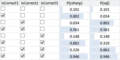
Inspecting this table, we can see that the results appear to be sensible – the probability of having the csharp skill is generally higher when the candidate got the first question correct and similarly the probability of having the sql skill is generally higher when the candidate got the second question correct. Also, both probabilities are higher when the third question is correct rather than incorrect.
Interestingly, the probability of having the sql skill is actually lower when only the first question is correct, than where the candidate got all the questions wrong (first and second rows of Table 2.4). This makes sense because getting the first question right means the candidate probably has the csharp skill, which makes it even more likely that the explanation for getting the third question wrong is that they didn’t have the sql skill. This is an example of the kind of subtle reasoning which model-based machine learning can achieve, which can give it an advantage over simpler approaches. For example, if we just used the number of questions needing a particular skill that a person got right as an indicator of that skill, we would be ignoring potentially useful information coming from the other questions. In contrast, using a suitable model, we have exploited the fact that getting a csharp question right can actually decrease the probability of having the sql skill.
inference queryA query which defines an inference calculation to be done on a probabilistic model. It consists of the set of variables whose values we know (along with those values) and another set of variables that we wish to infer posterior distributions for. An example of an inference query is if we may know that the variable weapon takes the value revolver and wish to infer the posterior distribution over the variable murderer.
product of distributionsAn operation which multiplies two (or more) probability distributions and then normalizes the result to sum to 1, giving a new probability distribution. This operation should not be confused with multiplying two different random variables together (which may happen using a deterministic factor in a model). Instead, a product of distributions involves two distributions over the same random variable. Products of distributions are used frequently during inference to combine multiple pieces of uncertain information about a particular variable which have come from different sources.
message passing algorithmAn algorithm for doing inference calculations by passing messages over the edges of a graphical model, such as a factor graph. The messages are probability distributions over the variable that the edge is connected to. Belief propagation is a commonly used message passing algorithm.
belief propagationA message passing algorithm for computing posterior marginal distributions over variables in a factor graph. Belief propagation uses two different messages computations, one for messages from factors to variables and one for messages from variables to factors. Observed variables send point mass messages. See Algorithm 2.1.
The following exercises will help embed the concepts you have learned in this section. It may help to refer back to the text or to the concept summary below.
- Compute the product of the following pairs of Bernoulli distributions
- Write a program (or create a spreadsheet) to print out pairs of samples from two Bernoulli distributions with different parameters and . Now filter the output of the program to only show samples pairs which have the same value (i.e. where both samples are true or where both are false). Print out the fraction of these samples which are true. This process corresponds to multiplying the two Bernoulli distributions together and so the resulting fraction should be close to the value given by equation (2.12).
Use your program to (approximately) verify your answers to the previous question. What does your program do when and ?
- Manually compute the posterior probability for the sql skill, as we did for the csharp skill in section 2.2, and show that it comes to 3.4%.
- Build this model in Infer.NET and reproduce the results in Table 2.4. For examples of how to construct a conditional probability table, refer to the wet grass/sprinkler/rain example in the Infer.NET documentation. You will also need to use the Infer.NET & operator for the And factor. This exercise demonstrates how inference calculations can be performed completely automatically given a model definition.
[Pearl, 1982] Pearl, J. (1982). Reverend Bayes on Inference Engines: A Distributed Hierarchical Approach. In Proceedings of the Second AAAI Conference on Artificial Intelligence, AAAI’82, pages 133––136. AAAI Press.
[Pearl, 1988] Pearl, J. (1988). Probabilistic Reasoning in Intelligent Systems. Morgan Kaufmann, San Francisco.
[Lauritzen and Spiegelhalter, 1988] Lauritzen, S. L. and Spiegelhalter, D. J. (1988). Local Computations with Probabilities on Graphical Structures and Their Application to Expert Systems. Journal of the Royal Statistical Society, Series B, 50(2):157–224.
[Bishop, 2006] Bishop, C. M. (2006). Pattern Recognition and Machine Learning. Springer.
[Kschischang et al., 2001] Kschischang, F. R., Frey, B. J., and Loeliger, H. (2001). Factor graphs and the sum-product algorithm. IEEE Transactions on Information Theory, 47(2):498–519.