1.2 Updating our beliefs

Searching carefully around the library, Dr Bayes spots a bullet lodged in the book case. “Hmm, interesting”, she says, “I think this could be an important clue”.

So it seems that the murder weapon was the revolver, not the dagger. Our intuition is that this new evidence points more strongly towards Major Grey than it does to Miss Auburn, since the Major, due to his age and military background, is more likely to have experience with a revolver than Miss Auburn. But how can we use this information?

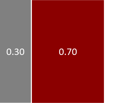
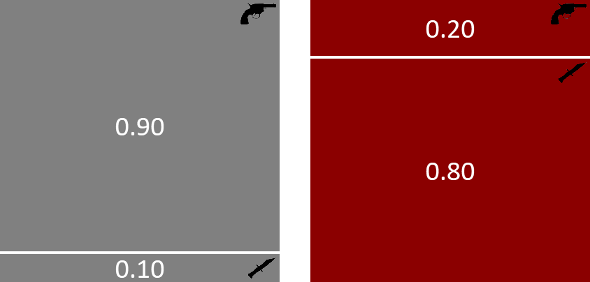
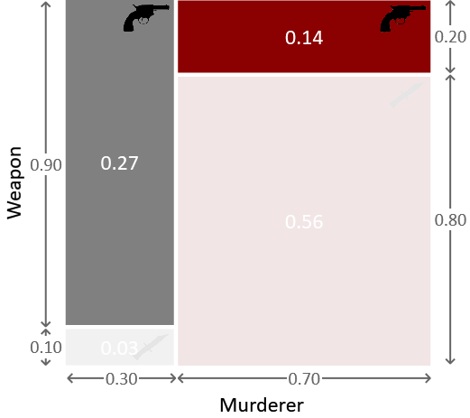
A convenient way to think about the probabilities we have looked at so far is as a description of the process by which we believe the murder took place, taking account of the various sources of uncertainty. So, in this process, we first pick the murderer with the help of Figure 1.2. This shows that there is a 30% chance of choosing Major Grey and a 70% chance of choosing Miss Auburn. Let us suppose that Miss Auburn was the murderer. We can then refer to Figure 1.4 to pick which weapon she used. There is a 20% chance that she would have used the revolver and an 80% chance that she would have used the dagger. Let’s consider the event of Miss Auburn picking the revolver. The probability of choosing Miss Auburn and the revolver is therefore 70% $\times$ 20% = 14%. This is the joint probability of choosing Auburn and revolver. If we repeat this exercise for the other three combinations of murderer and weapon we obtain the joint probability distribution over the two random variables, which we can illustrate pictorially as seen in Figure 1.5.

Figure 1.5Representation of the joint probabilities for the two random variables murderer and weapon.

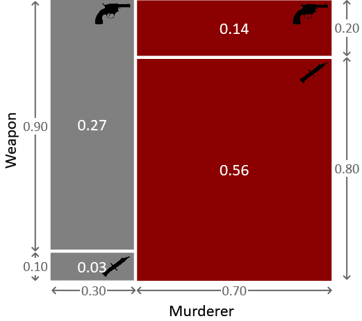
Figure 1.6 below shows how this joint distribution was constructed from the previous distributions we have defined. We have taken the left-hand slice of the $P(\var{murderer})$ square corresponding to Major Grey, and divided it vertically in proportion to the two regions of the conditional probability square for Grey. Likewise, we have taken the right-hand slice of the $P(\var{murderer})$ square corresponding Miss Auburn, and divided it vertically in proportion to the two regions of the conditional probability square for Auburn.

= $\times$ $P(\var{weapon}, \var{murderer})$   $P(\var{murderer})$   $P(\var{weapon} | \var{murderer})$

Figure 1.6The joint distribution for our two-variable model, shown as a product of two factors.

We denote this joint probability distribution by $P(\var{weapon}, \var{murderer})$, which should be read as “the probability of weapon and murderer”. In general, the joint distribution of two random variables A and B can be written $P(\var{A}, \var{B})$ and specifies the probability for each possible combination of settings of A and B. Because probabilities must sum to one, we have

Here the notation $\sum_A$ denotes a sum over all possible states of the random variable A, and likewise for B. This corresponds to the total area of the square in Figure 1.5 being 1, and arises because we assume the world consists of one, and only one, combination of murderer and weapon. Picking a point randomly in this new square corresponds to sampling from the joint probability distribution.

Two rules for working with joint probabilities

We’d like to use our joint probability distribution to update our beliefs about who committed the murder, in the light of this compelling new evidence. To do this, we need to introduce two important rules for working with joint distributions.

From the discussion above, we see that our joint probability distribution is obtained by taking the probability distribution over murderer and multiplying by the conditional distribution of weapon. This can be written in the form

Equation (1.15) is an example of a very important result called the product rule of probability. The product rule says that the joint distribution of A and B can be written as the product of the distribution over A and the conditional distribution of B conditioned on the value of A, in the form

Now suppose we sum up the values in the two left-hand regions of Figure 1.5 corresponding to Major Grey. Their total area is 0.3, as we expect because we know that the probability of Grey being the murderer is 0.3. The sum is over the different possibilities for the choice of weapon, so we can express this in the form

Similarly, the entries in the second column, corresponding to the murderer being Miss Auburn, must add up to 0.7. Combining these together we can write

This is an example of the sum rule of probability, which says that the probability distribution over a random variable A is obtained by summing the joint distribution $P(\var{A}, \var{B})$ over all values of B

In this context, the distribution $P(\var{A})$ is known as the marginal distribution for A and the act of summing out B is called marginalisation. We can equally apply the sum rule to marginalise over the murderer to find the probability that each of the weapons was used, irrespective of who used them. If we sum the areas of the top two regions of Figure 1.5 we see that the probability of the weapon being the revolver was $0.27 + 0.14 = 0.41$, or 41%. Similarly, if we add up the areas of the bottom two regions we see that the probability that the weapon was the dagger is $0.03 + 0.56 = 0.59$ or 59%. The two marginal probabilities then add up to $1$, which we expect since the weapon must have been either the revolver or the dagger.

The sum and product rules are very general. They apply not just when A and B are binary random variables, but also when they are multi-state random variables, and even when they are continuous (in which case the sums are replaced by integrations). Furthermore, A and B could each represent sets of several random variables. For example, if $\var{B} \equiv \{ \var{C}, \var{D} \}$, then from the product rule (1.16) we have

and similarly the sum rule (1.19) gives

The last result is particularly useful since it shows that we can find the marginal distribution for a particular random variable in a joint distribution by summing over all the other random variables, no matter how many there are.

Together, the product rule and sum rule provide the two key results that we will need throughout the book in order to manipulate and calculate probabilities. It is remarkable that the rich and powerful complexity of probabilistic reasoning is all founded on these two simple rules.

Inference using the joint distribution

We now have the tools that we need to incorporate the fact that the weapon was the revolver. Intuitively, we expect that this should increase the probability that Grey was the murderer but to confirm this we need to calculate that updated probability. The process of computing revised probability distributions after we have observed the values of some of the random variables, is called probabilistic inference. Inference is the cornerstone of model-based machine learning – it can be used for reasoning about a situation, learning from data, making predictions – in fact any machine learning task can be achieved using inference.

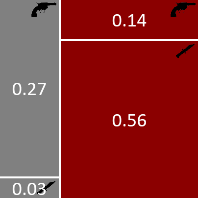
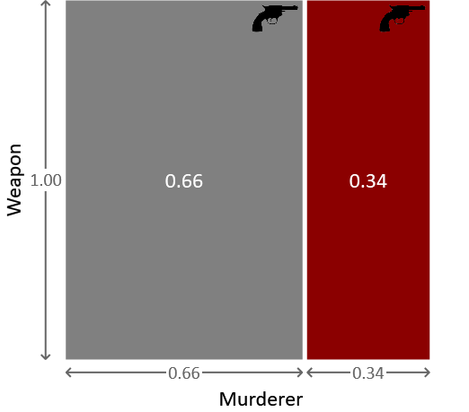
We can do inference using the joint probability distribution shown in Figure 1.5. Before we observe which weapon was used to commit the crime, all points within this square are equally likely. Now that we know the weapon was the revolver, we can rule out the two lower regions corresponding to the weapon being the dagger, as illustrated in Figure 1.7.

Figure 1.7This shows the joint distribution from Figure 1.5 in which the regions corresponding to the dagger have been eliminated.

Because all points in the remaining two regions are equally likely, we see that the probability of the murderer being Major Grey is given by the fraction of the remaining area given by the grey box on the left. $P(\var{murderer} = \state{Grey}| \var{weapon} = \state{revolver}) = \frac{0.27}{0.27 + 0.14} \simeq 0.66$ in other words a 66% probability. This is significantly higher than the 30% probability we had before observing that the weapon used was the revolver. We see that our intuition is therefore correct and it now looks more likely that Grey is the murderer rather than Auburn. The probability that we assigned to Grey being the murderer before seeing the evidence of the bullet is sometimes called the prior probability (or just the prior), while the revised probability after seeing the new evidence is called the posterior probability (or just the posterior).

The probability that Miss Auburn is the murderer is similarly given by $P(\var{murderer} = \state{Auburn}| \var{weapon} = \state{revolver}) = \frac{0.14}{0.27 + 0.14} \simeq 0.34.$ Because the murderer is either Grey or Auburn these two probabilities again sum to 1. We can capture this pictorially by re-scaling the regions in Figure 1.7 to give the diagram shown in Figure 1.8.

Figure 1.8Representation of the posterior probabilities that Grey or Auburn was the murderer, given that the weapon is the revolver.

We have seen that, as new data, or evidence, is collected we can use the product and sum rules to revise the probabilities to reflect changing levels of uncertainty. The system can be viewed as having learned from that data.

So, after all this hard work, have we finally solved our murder mystery? Well, given the evidence so far it appears that Grey is more likely to be the murderer, but the probability of his guilt currently stands at 66% which feels too small for a conviction. But how high a probability would we need? To find an answer we turn to William Blackstone’s principle [Blackstone, 1765]:

“Better that ten guilty persons escape than one innocent suffer.”

We therefore need a probability of guilt for our murderer which exceeds $\frac{10}{10+1} \approx 91\%$. To achieve this level of proof we will need to gather more evidence from the crime scene, and to make a corresponding extension to our joint probability in order to incorporate this new evidence. We’ll look at how to do this in the next section.