2.5 Diagnosing the problem

When a machine learning system is not working there are generally three possible reasons: bad data, bad model, or bad inference. Here are some common causes of problems under each of these three headings:

Bad data:

data items have been entered, stored or loaded incorrectly; the data items are incomplete or mislabelled; data values are too noisy to be useful; the data is biased or unrepresentative of how the system will be used; it is the wrong data for the task; there is insufficient data to make accurate predictions.

Bad model:

one or more of the modelling assumptions are wrong – that is, not consistent with the actual process that generated the data; the model makes too many simplifying assumptions; the model contains insufficient assumptions to make accurate predictions given the amount of available data.

Bad inference:

the inference code contains a bug; the message-passing schedule is bad; the inference has not converged; there are numerical problems (e.g. rounding, overflow); the approximate inference algorithm is not accurate enough.

In our case, we can be fairly confident that the data is good because we have inspected and visualised it carefully. So it seems likely that either the model or the inference is causing the problem. We’ll start by checking that the inference algorithm, loopy belief propagation, is working correctly.

Checking the inference algorithm

To see if inference is working correctly, we need to be able to separate out any problems caused by inference issues from any problems caused by our model not matching the data. To achieve this separation, we can generate a new synthetic data set which is guaranteed to match the model exactly. If we get poor results using this data set it suggests that there is an inference problem. We will create this synthetic data set by sampling from the joint distribution specified by the model, which guarantees that the data is consistent with the model (refer to Chapter 1 for a reminder of what sampling is). We can generate samples by running the data generation process specified by the model – a process called ancestral sampling, as defined by Algorithm 2.3 (see also Bishop [2006]).

Looking at the factor graph of Figure 2.19, we run ancestral sampling following the arrows from top to bottom (from ancestor to descendent), by sampling a value for each variable given its parents in the graph. If a variable is the child variable of a deterministic factor, then we just compute its value from the values of its parent variables using the function encoded by the deterministic factor (such as the $\mathrm{AND}$ function).

So, starting at the top, we sample a value for each element of the skill array from a Bernoulli(0.5) distribution – in other words we pick true with 50% probability and false otherwise. For the relevantSkills array element for a question we just pull out the already-sampled values of the skill array that are relevant to that question. These values are then ANDed together to give hasSkills. Figure 2.21 gives an example set of 22 samples for the skill and hasSkills arrays. To get a data set with multiple rows we just repeat the entire sampling process for each row. Notice how, for each row, hasSkills is always the same for questions that require the same skills (are the same colour).

Excel

CSV

(a)Sampled skill array

(b)hasSkills array computed from sampled skill array

 

(c)Sampled isCorrect array

Figure 2.21Synthetic data set created using ancestral sampling. First the skill array was sampled and then the hasSkill array was computed from it. The isCorrect array was then sampled given the hasSkill array, which has the effect of making it a noisy version of hasSkill.

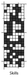
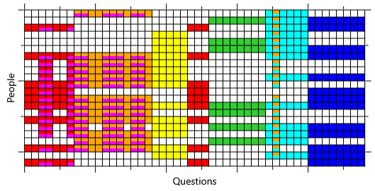
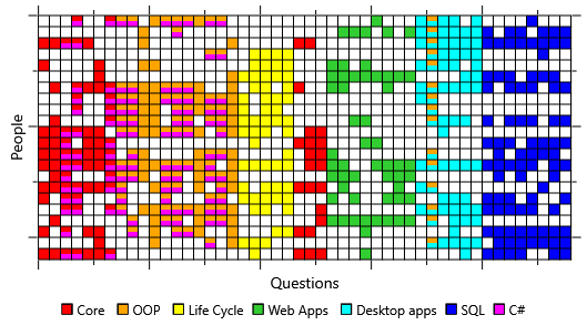
The final stage of ancestral sampling in our model requires sampling each element of isCorrect given its parent element of hasSkills. Where hasSkills is true we sample from Bernoulli(0.9) and where hasSkills is false we sample from Bernoulli(0.2) (following Table 2.1). The result of performing this step gives the isCorrect samples of Figure 2.21c. Notice that these samples end up looking like a noisy version of the hasSkills samples – about one in ten white squares has been flipped to colour and about one in five coloured squares has been flipped to white.

We now have an entire sampled data set, which we can run our inference algorithm on to test if it is working correctly. The inferred skill probabilities are shown in Figure 2.22 next to the actual skills that we sampled. Unlike with the real data, the results are pretty convincing: the inferred skills look very similar to the actual sampled skills. So, when we run inference on a data set that conforms perfectly to our model, the results are good. This suggests that the inference algorithm is working well and the problem must instead be that our model does not match the real data.

Excel

CSV

(a)Inferred skills

Excel

CSV

(b)Sampled skills

Figure 2.22Skills inferred from a sample data set shown next to the actual sampled skills for that data set. The inferred skills are close to the actual skills, suggesting that the inference algorithm is working well.

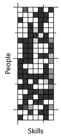
An important and subtle point is that the inferred skills are close but not identical to the sampled skills, even though the data is perfectly matched to the model. This is because there is still some remaining uncertainty in the skills even given all the answers in the test. For example, the posterior probability of skill 7 (C#) is uncertain in the cases where the individual does not have skill 1 (Core) or skill 2 (OOP). This makes sense because the C# skill is only tested in combination with these first two skills – if a person does not have them then they will get the associated questions wrong, whether or not they know C#. So in this case, the inference algorithm is correct to be uncertain about whether or not the person has the C# skill. We could use this information to improve the test, such as by adding questions that directly test the C# skill by itself.

Working out what is wrong with the model

We have determined that our model assumptions are not matching the data – now we need to identify which assumption(s) are at fault. We can again use sampling to achieve this but rather than sampling the skill array, we can set it to the true (self-assessed) values. If we then sample the isCorrect array, it will show us which answers the model is expecting people to get wrong if they had these skills. By comparing this to the actual isCorrect array from our data set, we can see where the model’s assumptions differ from reality. Figure 2.23 shows that the actual isCorrect data looks quite different to the sampled data.

(a)Sampled isCorrect array given true (self-assessed) skills

(b)Observed isCorrect array from our data set

Figure 2.23The modelling problem can be diagnosed by comparing (a) the isCorrect data sampled from the model given the self-assessed skills and (b) the observed isCorrect data showing which questions the volunteers actually got wrong.

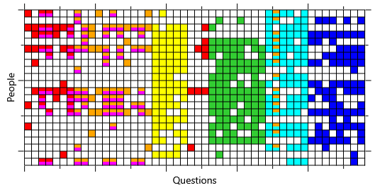
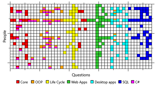
The biggest difference appears to be that our volunteers got many more questions right than our model is predicting, given their stated skills. This suggests that they are able to guess the answer to a question much more often than the 1-in-5 times that our model assumes. On reflection, this makes sense – even if someone doesn’t have the skill to answer a question they may be able to eliminate some answers on the basis of general knowledge or intelligent guesswork.

We can investigate this further by computing the fraction of times that our model predicts our volunteers should get each question right, given their self-assessed skills, and then compare it to the fraction of times they actually got it right (Figure 2.24).

Excel

CSV

Figure 2.24The fraction of people the model predicts will get each question right given their self-assessed skills (blue) compared to the fraction that actually got it right (red), for each of the 48 questions in the test.

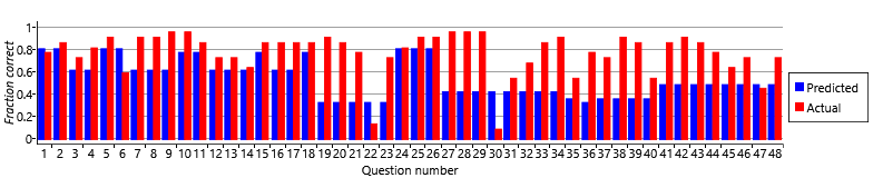
For a few questions, the fraction of people who got them correct matches that predicted by the model – but for most questions the actual fraction is higher than the predicted fraction. This suggests that some questions are easier to guess than others and that they can be guessed correctly more often than 1-in-5 times. So we need to change our assumptions (and our model) to allow different guess probabilities for different questions. We can modify our fourth assumption as follows:

4. If a candidate doesn’t have all the skills needed for a question, they will pick an answer at random guess an answer, where the probability that they guess correctly is about 20% for most questions but could vary up to about 60% for very guessable questions.

This assumption means that, rather than having a fixed guess probability for all questions, we need to extend our model to learn a different guess probability for each question.