-

Want a paper copy?
You can now buy the book!
All royalties go to the Cystic Fibrosis Trust.Spotted an error? Have comments?
Let us know!Get hands on with source code for the book.
7.2 Trying out the worker model
To try out the model, we must define some training and validation sets. For the validation set, we need to know the correct label, in order to be able to evaluate our model. So our validation set must consist only of tweets where we have gold labels. We will use 70% of the 950 gold labelled tweets as our validation set, so that some gold labels are available for training, if we want to use them. For the training set, we will use the remaining 30% of gold labelled tweets, plus a random selection of the remaining tweets to bring us to a totals of 20,000 tweets. The full statistics of the data sets are:
- Training set: 20,000 tweets with 54,440 labels from 1,788 workers;
- Validation set: 683 tweets with 3,637 labels from 764 workers.
To train our model, we will use the 20,000 training set tweets as our observed data. For now, we will not make any use of the gold labels during training. As we have throughout the book, we will use expectation propagation to infer posterior distributions over all unobserved variables.
For validation, we will apply the model to each validation tweet individually. The posteriors learned during training for the probability of each label probLabel and the ability of each worker will used as priors for these variables during validation. Expectation propagation will then be used to give posteriors over the trueLabel for the validation set tweet. The label with the highest probability under this posterior distribution will be considered to be the true label inferred by the model.
Since we have gold labels for all tweets in our validation set, we can use them to evaluate whether the inferred true label is correct. We can then compute the accuracy of our model, as the percentage of inferred labels that are correct. For this initial model, we find that our accuracy is 91.5%, which seems like a pretty good start!
Majority vote: the label with the most votes wins!
But before we break out the champagne, it would be helpful to know how good this accuracy really is. To do this, we should compare to a simple baseline method. We will use a simple method where the label assigned to a tweet is the one that the most workers chose, breaking ties at random. This method is called majority vote. If we use majority vote to label our validation set, then we get an accuracy of 90.3%. So, in fact, our model is giving us an improvement over this baseline, but only of 1.2%.
It’s informative to consider why our model is able to do better than majority vote. The main reason is that we are learning the abilities of each worker. This allows us to let the votes of good workers count more than the votes of bad workers. To explore this a bit more, let’s look at the inferred abilities of our workers. Figure 7.6 shows a histogram of the inferred abilities of our crowd workers.
 Excel
Excel CSV
CSV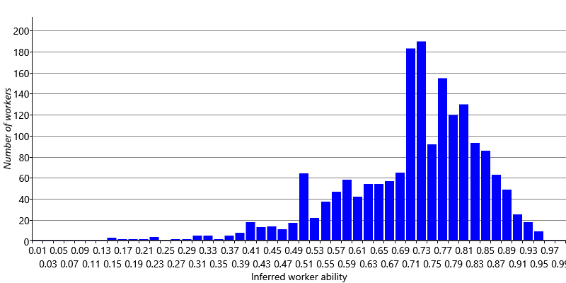
We can see from Figure 7.6 that almost all abilities are above , showing that most workers are able to provide correct labels – this is reassuring given that we assumed this in Assumptions0 7.5. The histogram also shows that there is a wide variety of abilities ranging from a bit over up to around . Being able to discount the weaker workers on the left of the histogram and pay more attention to the stronger workers on the right allows our model to achieve this 1.2% improvement in accuracy.
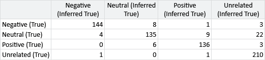
For our application, we want to push the accuracy as high as we can – as every correct label could have real benefit and every incorrect label could cause resources to be wasted. To increase our accuracy, it would be helpful to get a more detailed picture of the mistakes our model is making. If we had only two possible labels, we could count the true and false positives and the true and false negatives to produce a table in the structure of Table 2.7. In that table, each row corresponds to a true label and each column corresponds to an inferred label. Even though we have more than two labels, we can use the exact same table structure and put in each cell the count of tweets with the true label of the row and the inferred label of the column. This table is then called a confusion matrix. The confusion matrix for our initial model results is shown in Figure 7.7.
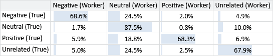
When working with a confusion matrix like this one, it can be hard to compare cells since the number of tweets with each true label varies. We can correct for this by dividing the value in each cell by the sum of the row and so express it as a percentage. A cell then shows the percentage of items with this true label that are predicted to have the particular inferred label. Figure 7.8 gives the same results as above expressed as a confusion matrix with percentages.
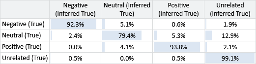
Looking at Figure 7.8, we can now see more clearly where the main sources of error are. For example, the most common error is that we are inferred the label Unrelated when the true label is Neutral. Another kind of error is incorrectly labelling Positive or Negative tweets as being Neutral – and, to a lesser extent, vice-versa.
Our model is making these errors because of labelling errors made by individual crowd workers. So, it would also be useful to understand the kinds of errors that particular crowd workers make by plotting a confusion matrix for each individual worker. The problem is that each worker labels relatively few tweets and it is likely that few, or even none, of these have gold labels. Instead of limiting ourselves to just gold labels, we can also use the inferred true label, as we expect that this will generally be more correct than any individual worker. The resulting confusion matrices will be an approximation, but hopefully a good enough for us to get insights into the kinds of errors that workers make.
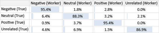
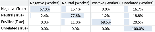
Figure 7.9 shows confusion matrices for three workers with different patterns of errors. For each of these three patterns, there were many workers with similar confusion matrices – we chose a representative example in each case. Figure 7.9a shows a worker who often gives the Neutral label to tweets that should have one of the other labels. Figure 7.9b shows a worker that makes relatively few mistakes – such a worker will have a high ability. Figure 7.9c shows a worker that often incorrectly gives the Unrelated label, while also giving the Neutral label to tweets that should be labelled as Positive or Negative.
Rather than just learn the overall ability of a worker, it would be helpful if we could learn the individual biases of the worker so that we can more accurately correct for different patterns of errors. We will look at how to do this in the next section.
baseline methodA method for doing a task that can be used to provide some comparative metrics. Such baseline metrics help us to understand just how good a model is at performing a task. We would generally hope that a new model would produce better metrics than a baseline model. If a model does not do much better than baseline then this suggests that either there is a bug in the model implementation or the model needs redesigning. A baseline method is often one that is simple to implement, so that not much effort is needed to run it and compute its metrics.
majority voteA method for labelling items where the winning label is the one with the most ‘votes’ – that is, the one that was given by the most crowd workers.
confusion matrixA table (matrix) giving the results of a label prediction problem. Each row of the table corresponds to a true label and each column of the table corresponds to a predicted label. The cells of the table then contain counts of items with the true label of the row and the inferred label of the column.
Here is an example confusion matrix, from Figure 7.7.