3.3 A solution: expectation propagation

We have seen that belief propagation allows us to calculate the exact marginal posterior distribution for the variable Jskill in the model of Figure 3.10. Whereas the prior distribution for Jskill is a Gaussian described by two parameters, the posterior distribution is not Gaussian but is a more complex distribution requiring four parameters. To stop the number of parameters increasing after every game, we need a way to approximate this true posterior by a distribution having a fixed number of parameters, and for this we choose the Gaussian. The posterior distribution will then have the same functional form as the prior, mimicking the behaviour of a conjugate prior. If we can achieve this, we will be able to treat the resulting approximate posterior distribution as the prior distribution for the next game. Then the skill for each player will always be represented by a Gaussian distribution governed by just two parameters.

The first question is how to approximate a non-Gaussian distribution by a Gaussian. A simple solution is to find the mean and the variance of the non-Gaussian distribution and then to choose as our approximation a Gaussian having the same mean and variance. This turns out to be a sensible approximation, which can be derived formally by optimizing a measure of the dissimilarity of two probability distributions [Bishop, 2006; Minka, 2005].

We might be tempted then just to approximate the exact posterior distribution for Jskill by a Gaussian. Although this will work satisfactorily for the factor graph of Figure 3.10 it will break down again as we go to more complex factor graphs (such as those we will encounter later in this chapter). Messages with simple functional forms tend to become more complex as a result of passing through factors. As we extend our model to larger and more sophisticated graphs we quickly arrive at situations where messages cannot be evaluated exactly. Such problems can be avoided by making our approximations locally at each factor node, so that all messages have the desired distribution type. This ensures that factors can be composed together into arbitrary graphs, as long as each factor is capable of sending approximate messages to all neighbouring variable nodes using the appropriate types of distribution.

The following section goes into the mathematical details of this kind of approximate inference algorithm. If you want to skip these details, feel free to go to the next section.

Inference deep-dive

In this optional section, we introduce the approximate inference technique of expectation propagation, which we will use extensively in this book. If you want to focus on modelling, feel free to skip this section.

Returning to Figure 3.12 (which is reproduced in Figure 3.21 for convenience), we see that message (6) was the first message that we encountered which was non-Gaussian.

(5) (9) (8) (1) (2) (7) (6) (3) (4) observed bool variable Whether Jill won the game Jwins=T double variable Jill's skill Jskill double variable Fred's skill Fskill double variable Jill's performance Jperf double variable Fred's performance FperfGaussian(120, 40²)Gaussian(100, 5²)Gaussian(•, 5²)Gaussian(•, 5²)>

Figure 3.21The messages which arise in the application of belief propagation to the evaluation of the updated distribution for Jskill. (Reproduced from Figure 3.12.)

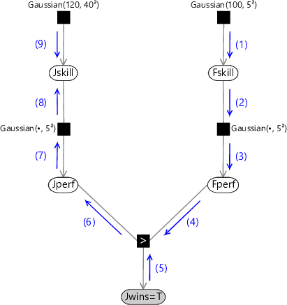
Our goal is therefore to approximate message (6) by a Gaussian, thereby ensuring that all subsequent messages will also be Gaussian distributions.

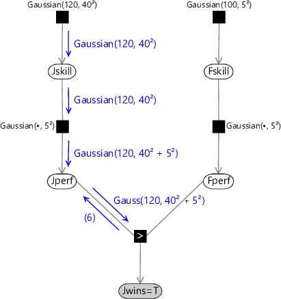
While this seems like a desirable goal, there also seems to be a significant obstacle – the exact form of message (6) as seen in Figure 3.17 does not look at all Gaussian! In fact, its mean and variance are not even well defined (they are both infinite). The key to finding a sensible Gaussian approximation is to notice that the approximate version of message (6) will subsequently be passed through the graph as modified forms of messages (7) and (8) and will then be multiplied by the downward message (9) in order to determine the (approximate) posterior distribution of Jskill. Our goal will therefore be to make the Gaussian approximation to message (6) over Jperf be most accurate in those regions which are considered more probable by the information coming from other parts of the graph. As we have just discussed, however, we need to keep our approximation local to the region of the graph where the message is generated. Message (6) is sent to the node Jperf and so we can choose our approximation so as to maximize the accuracy of the marginal distribution of Jperf. This is obtained by multiplying message (6) by the downward message on the same edge in the graph, which can be evaluated as shown in Figure 3.22. Note that these same messages are needed to find the posterior marginal for Fskill, so there is no additional overhead introduced by evaluating them.

Gaussian(120, 40²) Gaussian(120, 40²) Gaussian(120, 40² + 5²) Gauss(120, 40² + 5²)(6) observed bool variable Whether Jill won the game Jwins=T double variable Jill's skill Jskill double variable Fred's skill Fskill double variable Jill's performance Jperf double variable Fred's performance FperfGaussian(120, 40²)Gaussian(100, 5²)Gaussian(•, 5²)Gaussian(•, 5²)>

Figure 3.22Evaluation of the context message that will be used to find a Gaussian approximation for message (6).

Let’s consider the piece of the factor graph close to the Jperf node in more detail, as seen in Figure 3.23.

ce (CumGauss) observed bool variable Whether Jill won the game Jwins=T double variable Jill's skill Jskill double variable Fred's skill Fskill double variable Jill's performance Jperf double variable Fred's performance FperfGaussian(120, 40²)Gaussian(100, 5²)Gaussian(•, 5²)Gaussian(•, 5²)>

(a)

  

cg (Gaussian) observed bool variable Whether Jill won the game Jwins=T double variable Jill's skill Jskill double variable Fred's skill Fskill double variable Jill's performance Jperf double variable Fred's performance FperfGaussian(120, 40²)Gaussian(100, 5²)Gaussian(•, 5²)Gaussian(•, 5²)>

(b)

Figure 3.23Detail of the factor graph around the Jperf node, showing the messages involved (a) when running belief propagation (b) when making a local Gaussian approximation to the upward message from the GreaterThan factor.

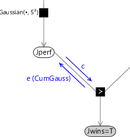
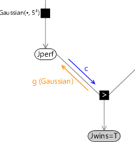
Here $e$ denotes the exact message (6) as seen previous in Figure 3.20, $c$ denotes the downward ‘context’ message, and $g$ denotes our desired Gaussian approximation to message $e$. These messages are all just functions of the variable Jperf. We have already seen that we cannot simply approximate message $e$ by a Gaussian since message $e$ has infinite mean and variance. Instead we make a Gaussian approximation for the marginal distribution of Jperf. The exact marginal is given by the product of incoming messages $ce$. We therefore define our approximate message $g$ to be such that the product of the messages $c$ and $g$ gives a marginal distribution for Jperf which is a best Gaussian approximation to the true marginal, so that

$$\begin{equation} cg = \mbox{Proj} \left( c e \right). \label{eq:EP-approx-marginal} \end{equation}$$

Here Proj() denotes ‘projection’ and represents the process of replacing a non-Gaussian distribution with a Gaussian having the same mean and variance. This can be viewed as projecting the exact message onto the ‘nearest’ message within the family of Gaussian distributions. Dividing both sides by $c$ we then obtain

$$\begin{equation} g = \frac{\mbox{Proj} \left( c e \right) }{ c }. \label{eq:EP-approx-message} \end{equation}$$

Details of the mathematics of how to do this are discussed in Herbrich et al. [2007].

We therefore find a Gaussian approximation $g$ to the exact $e$ message (6) as follows. First we compute the exact outgoing message (6) as before. This is shown in blue in Figure 3.24.

Excel

CSV

Figure 3.24Plot of the exact outgoing message (6) in blue, the incoming $\dist{Gaussian}(120, 40^2 + 5^2)$ context message in red, and the product of these two messages in green.

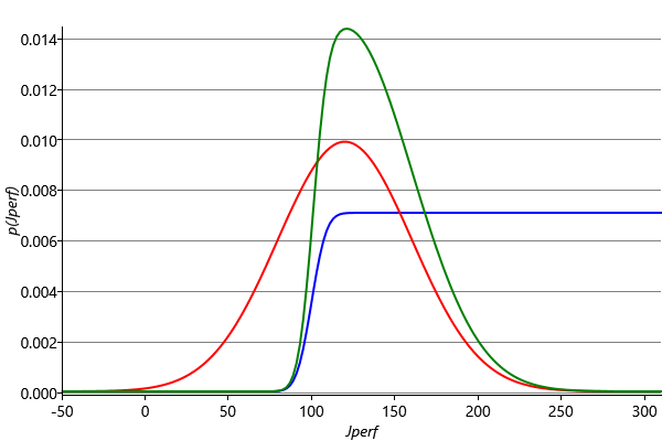
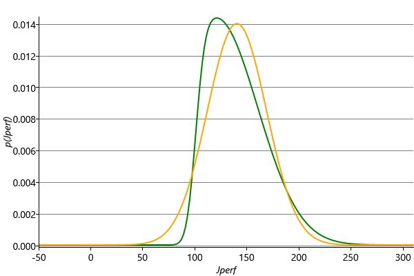
Then we multiply this by the incoming message context message $c$ which is shown in red in Figure 3.24. This gives a distribution, shown in green in Figure 3.24 which is non-Gaussian but which is localised and therefore has finite mean and variance and so can be approximated by a Gaussian. This curve is repeated in Figure 3.25 which also shows the Gaussian distribution which has the same mean and variance.

Excel

CSV

Figure 3.25In green, the product of the true belief propagation and incoming context messages copied from Figure 3.24. In orange, the Gaussian approximation to this product, which is $\dist{Gaussian}(140.4, 28.5^2)$.

Finally, we divide this Gaussian distribution by the incoming Gaussian context message $c$ to generate our approximate outgoing $g$ message. Because the ratio of two Gaussians is itself a Gaussian [Bishop, 2006], the resulting outgoing message will also be Gaussian, which was our original goal. For our specific example, this message is a Gaussian with mean $160.8$ and standard deviation $40.2$. The computation of the approximate message is summarised in Figure 3.26.

Excel

CSV

Figure 3.26The steps involved in computing the Gaussian approximation to message (6). The blue curve shows the exact message (6), the red curve shows the incoming context message $\dist{Gaussian}(120, 40^2 + 5^2)$, the orange curve shows the Gaussian approximation to the product of true message and context message which is $\dist{Gaussian}(140.4, 28.5^2)$. Finally, the purple curve shows the result of dividing the orange curve by the red context message to give $\dist{Gaussian}(160.8, 40.2^2)$. This Gaussian is then used as message (6).

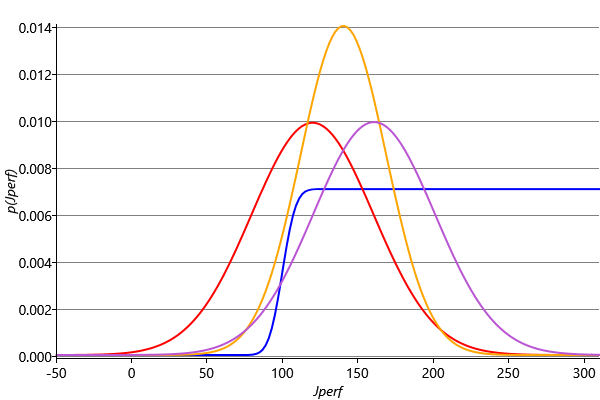
We see that overall we multiplied by the incoming context message, then made the Gaussian approximation, then finally divided out the context message again. The evidence provided by the incoming message is therefore used only to determine the region over which the Gaussian approximation should be accurate, but is not directly incorporated into the approximated message. If we happened to have a conjugate distribution, then the projection operation would be unnecessary and the context message would have no effect.

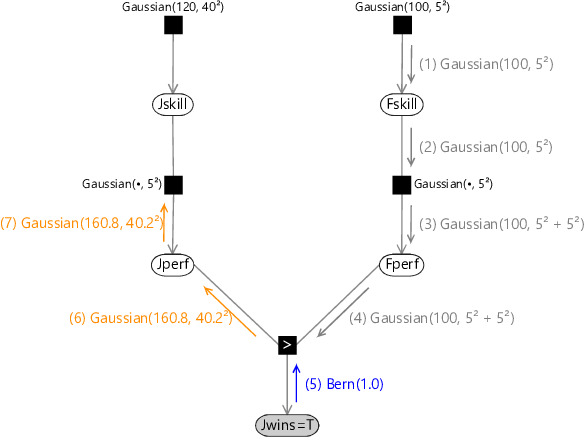
Now that we have found a suitable Gaussian approximation to the outgoing message (6) we can continue to pass messages along the graph to give the corresponding approximate message (7) as shown in Figure 3.27.

(5) Bern(1.0)(1) Gaussian(100, 5²)(2) Gaussian(100, 5²)(6) Gaussian(160.8, 40.2²)(3) Gaussian(100, 5² + 5²)(4) Gaussian(100, 5² + 5²)(7) Gaussian(160.8, 40.2²) observed bool variable Whether Jill won the game Jwins=T double variable Jill's skill Jskill double variable Fred's skill Fskill double variable Jill's performance Jperf double variable Fred's performance FperfGaussian(120, 40²)Gaussian(100, 5²)Gaussian(•, 5²)Gaussian(•, 5²)>

Figure 3.27Messages (5), (6), and (7) in the evaluation of the updated distribution for Jskill. Note that messages (6) and (7), which are highlighted in orange, differ from the exact messages in Figure 3.18.

Evaluation of the new (approximate) version of message (8) again involves the convolution of a Gaussian with a Gaussian, with the result shown in Figure 3.28.

(5) Bern(1.0)(8) Gaussian(160.8, 40.5²)(1) Gaussian(100, 5²)(2) Gaussian(100, 5²)(7) Gaussian(160.8, 40.2²)(6) Gaussian(160.8, 40.2²)(3) Gaussian(100, 5² + 5²)(4) Gaussian(100, 5² + 5²)(9) Gaussian(120, 40²) observed bool variable Whether Jill won the game Jwins=T double variable Jill's skill Jskill double variable Fred's skill Fskill double variable Jill's performance Jperf double variable Fred's performance FperfGaussian(120, 40²)Gaussian(100, 5²)Gaussian(•, 5²)Gaussian(•, 5²)>

Figure 3.28Messages (8) and (9) in the evaluation of the updated distribution for Jskill. Note that in addition to messages (6) and (7), message (8) (in orange) also differs from the exact message from Figure 3.19.

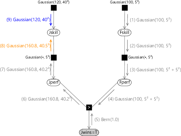
The downward message (9) is unchanged, and so we can finally compute the Gaussian approximation to the posterior distribution of Jskill as the product of two Gaussians, which gives the final result of a Gaussian with mean 140.1 and standard deviation 28.5.

This approach to locally approximate messages during the message-passing process is known as expectation propagation (or EP) and was developed by Minka [2001]. The approximation is being made locally at the factor node, and in a way that is independent of the structure of the remainder of the graph. This technique can therefore be applied to arbitrarily structured graphs, so long as each factor is consistently sending and receiving messages with the required distribution types, in this case Gaussians. The expectation propagation algorithm is summarised in Algorithm 3.1 with the differences to loopy belief propagation highlighted in red.

Applying expectation propagation

Let’s see what happens to the skill distributions when we apply expectation propagation to our game of Halo between Jill and Fred. First we suppose that Jill is the winner of the game. In Figure 3.29 we see the prior (dashed) and posterior (solid) distributions of skill for Jill and Fred.

Excel

CSV

Figure 3.29The result of applying the TrueSkill model for a game between Jill (blue) and Fred (red) for the case where Jill is the winner. The prior distributions are shown as dashed curves, and the corresponding posterior distributions are shown as solid curves. Jill’s initial broad skill distribution says that, before the game, we did not know if Jill was more or less skilled than Fred. After seeing that she won the game, her skill distribution shifts so that most of the area is to the right of Fred’s curve, meaning that we now think is it likely that Jill is more skilled than Fred. Because we were already relatively confident about Fred’s skill level, his distribution barely changes at all.

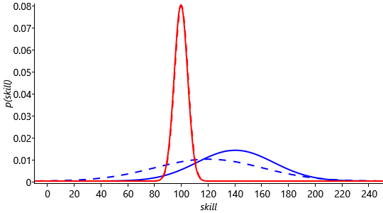
Because Jill is the winner, the mean of the skill distribution for Jill increases, while the mean of the skill distribution for Fred decreases. The increase in mean is quite large for Jill, whereas the mean for Fred hardly decreases at all. This difference is due to the greater certainty in Fskill compared to that for Jskill. Intuitatively we are using the more certain skill of Fred to estimate the skill of Jill. We also see from Figure 3.29 that the standard deviation for Jill’s skill distributions decreases as a result of this game. This is because we have learned something about her skill and therefore the degree of uncertainty is reduced.

Alternatively, if Fred were to have won the game, we have the results shown in Figure 3.30,

Excel

CSV

Figure 3.30As in Figure 3.29 but for the case where Fred is the winner. The prior distributions (dashed lines) are the same as before. Again our belief about Fred’s skill barely changes. But now Jill’s posterior skill distribution is shifted so that most of the area is to the left of Fred’s curve, meaning that we now think Jill is less skilled than Fred.

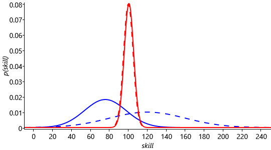
This result is slightly more surprising, since we believed Jill to be the stronger player, although we were not confident about this. Intuitively we would expect the adjustments of the skill distributions therefore to be slightly greater, which is indeed the case. We see that the shift in the means of the distributions is larger than in Figure 3.29. In fact the change in the mean of the distribution of Jskill is so large that it is now less than the mean of Fskill. Again, the standard deviations of Jill’s skill has decreased, reflecting a reduction in uncertainty due to the incorporation of new evidence. Because the skill updates in TrueSkill model depend on the variance of the skill distribution, TrueSkill is able to make relatively large changes to the distributions of new players. Furthermore, this happens automatically as a consequence of running inference in our model.

Multiple games

So far in this section we have developed a probabilistic model for a single game of Halo between Jill and Fred. In practice we will have a large pool of players, and individual games will take place between pairs of players from within that pool. When we try to assess the skill of a player we potentially have available the results of all the games ever played by that player against a range of different opponents. We might also have available the results of all the games played by those opponents, many of which might involve yet other players, and so on. In principle, all of this information is relevant and could help us to assess the original player’s skill. Furthermore, every time there is a new game outcome we could include this additional information and update the skill of the player even if they themselves haven’t played any new games. This new information could be relevant even if it involves a game between other players since it could influence the assessment of their skills, and hence the relative skill of our player.

We could in principle handle this by constructing a very large factor graph expressing all of the games played so far. Each player would have a single variable representing their skill value, but multiple variables (one for each game they have played) representing their performances on each of the games. This would be a complex graph with multiple loops, and we could run (loopy) expectation propagation, to keep the messages within the Gaussian family of distributions, until a suitable convergence criterion is satisfied. This would give a posterior skill distribution for each of the players, taking account of all of the games played. If a new game is then played we would start again with a new, larger factor graph and re-run inference in order to obtain the new posterior distributions of every player. This approach would be complex to implement and would get increasingly slow with each new game added. With millions of games being played each day, it is completely infeasible.

Instead we can use an approximate inference approach known as online learning (sometimes called filtering) in which each player’s skill distribution gets updated only when a game outcome is obtained which involves that player. We therefore need only store the mean and variance of the Gaussian skill distribution for each player. When a player plays a new game, we run inference using this current Gaussian skill distribution as the prior, and the resulting posterior distribution is then stored and forms the prior for the next game. Each single game is therefore described by a graph of the form shown in Figure 3.10.

This particular form of online inference algorithm, based on local projection onto the Gaussian distribution in which each data point (i.e. game outcome) is used only once, is also known as Gaussian Density Filtering [Maybeck, 1982; Opper, 1998]. It can be viewed as a special case of expectation propagation in which a specific choice is made for the message-passing schedule: namely that messages are only passed forwards in time from older games to newer games, but never in the reverse direction.

It is worth noting that, if we consider the full factor graph describing all games played so far, then the order in which those games had been played would have been irrelevant. When doing online learning, however, the ordering becomes significant and can influence the assessed skills. We have to live with this, however, as only online learning would be feasible in a practical system.

We can illustrate the behaviour of online learning in our model using data taken from the game Halo 2 on Xbox Live. We use a data set involving 1,650 players which contains the outcomes of 5,915 games. Each game is a head-to-head contest in which a pair of players play against each other. Figure 3.31 shows how the skill distributions for two of the top players varies as a function of the number of game outcomes played by each of the two players. To fit our model, these results ignore games which ended in a draw – we will see how to handle drawn games later in the chapter.

Excel

CSV

Figure 3.31Trajectories of skill distributions of two of the top players in the Halo2 head-to-head dataset, showing the mean and the one-standard-deviation envelopes. The horizontal axis shows the number of games played by the corresponding player.

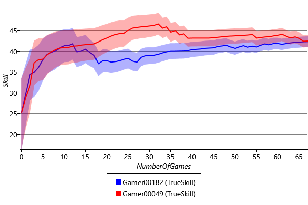
We see that the initial skill distributions are the same, because all player skills have the same prior distribution before any games are played. As an increasing number of games are played, we see that the standard deviation of the skill distributions decreases. This reduction in uncertainty as a result of observing the outcome of games is the effect we saw earlier in Figure 3.29 and Figure 3.30.

The model we have constructed in this section represents a single game between two players. However, many games on Xbox Live have a more elaborate structure, and so we turn next to a number of model extensions which allow for these additional complexities.