5.1 Learning about people and movies

The goal of this chapter is to make personalized movie recommendations to particular people. One way to think about this problem is to imagine a table where the rows are movies and the columns are people. The cells of the table show whether the person likes or dislikes the movie – for example, as shown in Table 5.1. This table is an illustration of the kind of data we might have to train a recommender system, where we have asked a number of people to say whether they like or dislike particular movies.

Table 5.1A table showing the kind of data used to train a recommender system. Each row is a movie and each column is a person. Filled cells show where a person has said that they liked or disliked a movie. Empty cells show where we do not have any information about whether the person liked the movie, and so are where we could make a like/dislike prediction. Making such a prediction for every empty cell in a person’s column would allow us to make a movie recommendation for that person – for example, by recommending the movie with the highest probability that the person would like it.

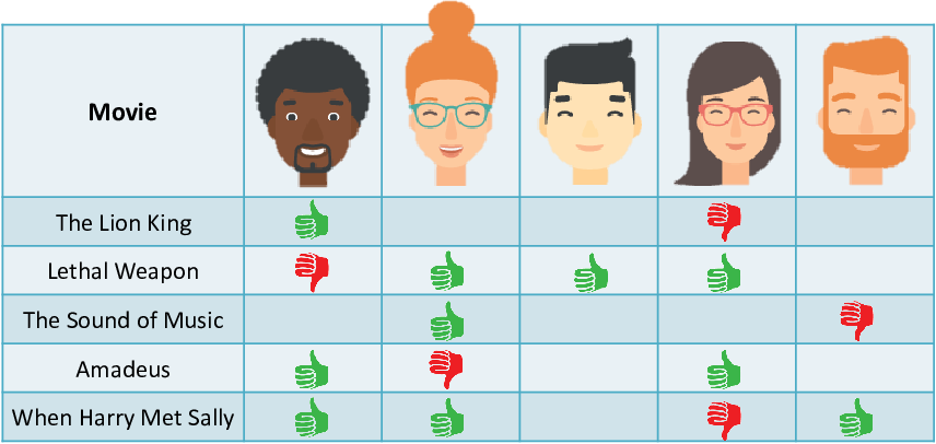
The empty cells in Table 5.1 show where we do not know whether the person likes the movie or not. There are bound to be such empty cells – we cannot ask every person about every movie and, even if we did, there will be movies that a person has not seen. The goal of our recommender system can be thought of as filling in these empty cells. In other words, given a person and a movie, predict whether they will like or dislike that movie. So how can we go about making such a prediction?

Characterizing movies

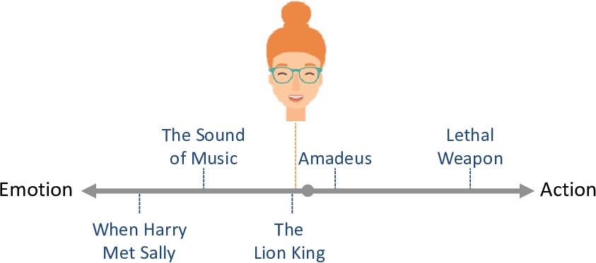
Let’s start by considering how to characterize a movie. Intuitively, we can assume that each movie has some traits, such as whether it is an escapist or realistic, action or emotional, funny or serious. If we consider a particular trait as a line, we can imagine placing movies on that line, like this:

Figure 5.2Movies placed on a line representing how much each movie is an emotional movie or as an action movie (or neither).

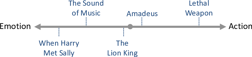
Movies towards the left of the line are emotional movies, like romantic comedies. Movies towards the right of the line are action movies. Movies near the middle of the line are neutral – neither action movies nor emotional movies. Notice that, in defining this trait, we have made the assumption that action and emotional are opposites.

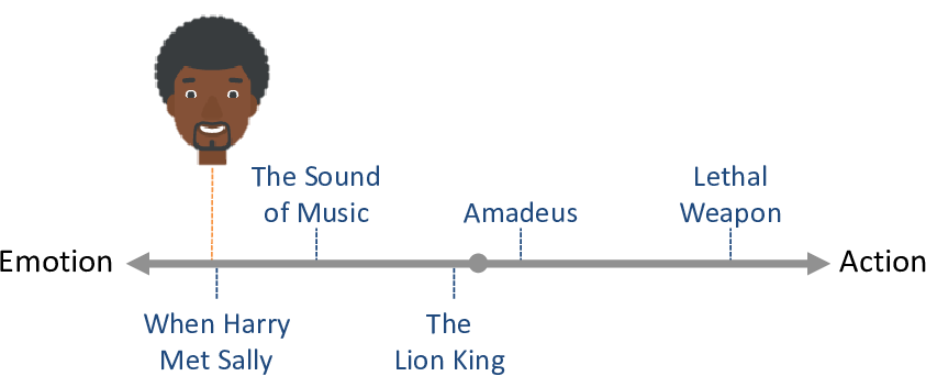
Now let’s consider people. A particular person might like emotional movies and dislike action movies. We could place that person towards the left of the line (Figure 5.3). We would expect such a person to like movies on the left-hand end of the line and dislike movies on the right-hand end of the line.

Figure 5.3A person placed on the left of the line would be expected to like emotional movies and dislike action movies.

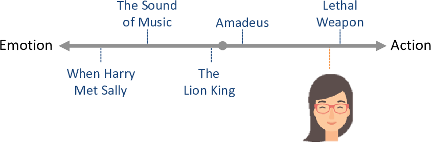
Another person may have the opposite tastes: disliking emotional movies and loving action movies. We can place this person towards the right of the line (Figure 5.4). We would expect such a person to dislike movies on the left-hand end of the line and like movies on the right-hand end of the line.

Figure 5.4A person placed on the right of the line would be expected to like action movies and dislike emotional movies.

It is also perfectly possible a person to like (or dislike) both action and emotional movies. We could consider such a person to be neutral to the action/emotion trait and place them in the middle of the line (Figure 5.5). We would expect that such a person might like or dislike movies anywhere on the line.

Figure 5.5A person placed in the middle of the line, would be expected to not care whether a movie was an action movie or an emotional one.

We’d like to use an approach like this to make personalized recommendations. The problem is that we do not know where the movies lie on the line or where the people lie on the line. Luckily, we can use model-based machine learning to infer both of these using an appropriate model.

A model of a trait

Let’s build a model for the action/emotion trait we just described. First, let’s state some assumptions that follow from the description above:

1. Each movie can be characterized by its position on the trait line, represented as a continuous number.
2. A person’s preferences can be characterized by a position on the trait line, again represented as a continuous number.

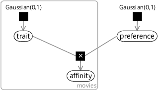
In our model, we will use a trait variable to represent the position of each movie on the trait line. Because it is duplicated across movies, this variable will need to lie inside a movies plate. We also need a variable for the position of the person on the line, which we will call preference since it encodes the person’s preferences with respect to the trait. To make predictions, we need a variable showing how much the person is expected to like each movie. We will call this the affinity variable and assume that a positive value of this variable means that we expect the person to like the movie and a negative value means that we expect the person to dislike the movie.

We need a way to combine the trait and the preference to give the behaviour described in the previous section. That is, a person with a negative (left-hand end) preference should prefer movies with negative (left-hand end) trait values. A person with a positive (right-hand end) preference should prefer movies with positive (right-hand end) trait values. Finally, a neutral person with a preference near zero should not favour any movies, whatever their trait values. This behaviour can be summarised as an assumption:

3. A positive preference value means that a person prefers movies with positive values of the trait (and vice versa for negative values). The absolute size of the preference value indicates the strength of preference, where zero means indifference.

This behaviour assumption can be encoded in our model by defining affinity to be the product of the trait and the preference. So we can connect these variables using a product factor, giving the factor graph of Figure 5.6.

plate of size: movies movies double variable The person's preference for this trait (their position on the trait line). preference double[] variable The movie's trait value (its position on the trait line). trait double variable The affinity that the person has for each movie (more positive means higher probability that they will like the movie). affinityGaussian(0,1)Gaussian(0,1)×

Figure 5.6Factor graph for a single trait. Each movie has a trait value which is multiplied by the person’s preference to give their affinity for that movie. More positive affinity values mean that the person is more likely to like the movie.

If you have a very good memory, you might notice that this factor graph is nearly identical to the one for a one-feature classifier (Figure 4.1) from the previous chapter. The only difference is that we have an unobserved trait variable where before we had an observed featureValue. In a way, we can think of our recommendation model as learning the features of a movie based on people’s likes and dislikes – a point we will discuss more later. As we construct our recommendation model, you will see that it is similar in many ways to the classification model from Chapter 4.

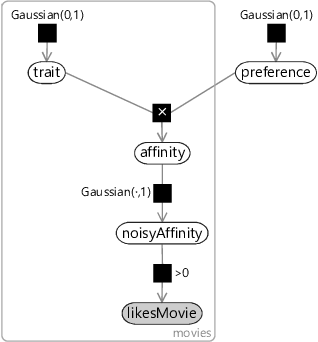
Given this factor graph, we want to infer both the movies’ trait values and the person’s preference from data about the person’s movie likes and dislikes. To do any kind of learning we need to have some variable in the model that we can observe – more specifically, we need a binary variable that can take one of two values (like or dislike). Right now we only have a continuous affinity variable rather than a binary one. Sounds familiar? Yes! We encountered exactly this problem back in section 4.2 of the previous chapter, where we wanted to convert a continuous score into a binary reply prediction. Our solution then was to add Gaussian noise and then threshold the result to give a binary variable. We can use exactly the same solution here by making a noisy version of the affinity (called noisyAffinity) and then thresholding this to give a binary likesMovie variable. The end result is the factor graph of Figure 5.7 (which closely resembles Figure 4.4 from the last chapter).

plate of size: movies movies observed bool variable Whether the person likes the movie. likesMovie double variable The person's preference for this trait (their position on the trait line). preference double[] variable The movie's trait value (its position on the trait line). trait double variable The affinity that the person has for each movie (more positive means higher probability that they will like the movie). affinity double variable Noisy version of the affinity, to allow for uncertainty in whether a person likes a movie. noisyAffinityGaussian(0,1)Gaussian(0,1)×Gaussian(·,1)>0

Figure 5.7Extended factor graph that converts the continuous affinity into a binary likesMovie variable, which can be observed to train the model.

We could start using this model with one trait and one person, but that wouldn’t get us very far – we would only learn about the movies that the person has already rated and so would only be able to recommend movies that they have already seen. In the next section, we will extend our model to handle multiple traits and multiple people so that we can characterise movies more accurately and use information from many peoples’ ratings pooled together, to provide better recommendations for everyone.