-

Want a paper copy?
You can now buy the book!
All royalties go to the Cystic Fibrosis Trust.Spotted an error? Have comments?
Let us know!Get hands on with source code for the book.
5.4 Our first recommendations

With our trained two-trait model in hand, we are now ready to make some recommendations! During training we learned the (uncertain) position of each movie and each person in trait space. We can now make a prediction for each of the held out ratings in our validation set. We do this one rating at a time – that is, for one person and one movie at a time. First, we set the priors for the movie trait and the person preference to the posteriors learned during training. Then we run expectation propagation to infer the posterior distribution over likesMovie to compute the probability that the person would like the movie. Repeating this over all ratings in the validation set gives a probability of ‘like’ for each rating, which we can compare with the ground truth like/dislike label. Figure 5.15 shows the predicted like probability and the ground truth for the ratings from the first 25 people in the validation set with more than five ratings.
 Excel
Excel CSV
CSV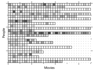
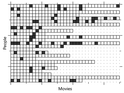
The first thing that stands out from Figure 5.15b is that people mostly like movies, rather than dislike them. In a sense then, the task that we have set our recommender is to try and work out which are the few movies that a person does not like. Looking at the predicted probabilities in Figure 5.15a, we can see some success in this task – because some of the darker squares do correctly align with black squares in the ground truth. In addition, some rows are generally darker or lighter than average indicating that we are able to learn how likely each person is to like or dislike movies in general. However, the predictions are not perfect – there are many disliked movies that are missed and some predictions of dislike that are incorrect. But before we make any improvements to the model, we need to decide which evaluation metrics we will use to measure and track these improvements.
Evaluating our predictions
In order to evaluate these predictions, we need to decide on some evaluation metrics. As discussed in Chapter 2, it makes sense to consider multiple metrics to avoid falling into the trap described by Goodhart’s law. For the first metric, we will just use the fraction of correct predictions, when we predict the most probable value of likesMovie. For the two-trait experiment above, we see that we get 84.8% of predictions correct. This metric is helpful for tracking the raw accuracy of our recommender but it does not directly tell us how good our recommendation experience will be for users. To do this, we will need a second metric more focused on how the recommender will actually be used.
The most common use of a recommender system is to provide an ordered list of recommendations to the user. We can use our predicted probabilities of ‘like’ to make such a list by putting the movie with the highest probability first, then the one with the second highest probability and so on. In this scenario, a reasonable assumption is that the user will scan through the list looking for a recommendation that appeals – but that they may give up at some point during this scan. It follows that it is most important that the first item in the list is correct, then the second, then the third and so on through to the end of the list. We would like to use an evaluation metric which rewards correct predictions at the start of the list more than at the end (and penalises mistakes at the start of the list more than mistakes at the end).
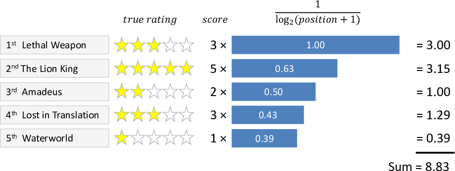
A metric that has this behaviour is Discounted Cumulative Gain (DCG) which is defined as the sum of scores for individual recommendations, each weighted by a discount function that depends on the position of the recommendation in the list. Figure 5.16 shows the calculation of DCG for a list of five recommendations. In this figure, the discount function used is where the position in the list, starting at 1. This function is often used because it smoothly decreases with list position, as shown by the blue bars in the figure. The score that we will use for a recommendation is the ground truth number of stars that the person gave that movie. So if they gave three stars then the score will be 3. Since we are calculating DCG for a list of five recommendations, we sometimes write this as DCG@5.
We can only evaluate a recommendation when we know the person’s actual rating for the movie being recommended. For our data set, this means that we will only be able to make recommendations for movies from the 30% of ratings in the validation set. Effectively we will be ordering these from ‘most likely to like the movie’ to ‘least likely to like the movie’, taking the top 5 and using DCG to evaluate this ordering.
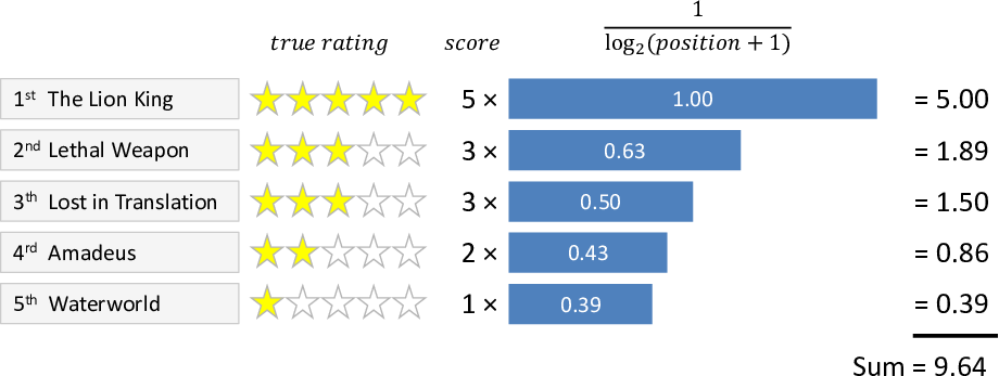
One problem with DCG is that the maximum achievable value varies depending on the ratings that the person gave to the validation set movies. If there are 5 high ratings then the maximum achievable DCG@5 will be high. But if there are only 2 high ratings then the maximum achievable DCG@5 will be lower. To interpret the metric, all we really want to know is how close we got to the maximum achievable DCG. We can achieve this by computing the maximum DCG (as shown in Figure 5.17) and then dividing our DCG value by this maximum possible value. This gives a new metric called the Normalized Discounted Cumulative Gain (NDCG). An NDCG of 1.0 always means that the best possible set of recommendations were made. Using the maximum value from Figure 5.17, the NDCG for the recommendations in Figure 5.16 is equal to .
We produce a list of recommendations for each person in our validation set, and so can compute an NDCG for each of these lists. To summarise these in a single metric, we then take an average of all the individual NDCG values. For the experiment we just ran, this gives an average NDCG@5 of 0.857.
How many traits should we use?
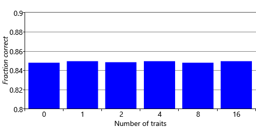
The metrics computed above are for a model with two traits. In practice, we will want to use the number of traits that gives the best recommendations according to our metrics. We can run the model with 1, 2, 4, 8, and 16 traits to see how changing the number of traits affects the accuracy of our recommendations. We can also run the model with zero traits, meaning that it gives the same recommendations to everyone – this provides a useful baseline and indicates how much we are gaining by using traits to personalise our recommendations to individual people. Note that when using zero traits, we do still include the movie and user biases in the model.
Figure 5.18 shows how our two metrics vary as we change the number of traits. Looking at the like/dislike accuracy in Figure 5.18a, shows that the accuracy is essentially unchanged as we change the number of traits. But the NDCG in Figure 5.18b tells a very different story , with noticeable gains in NDCG@5 as we increase the number of traits up to around 4 or 8. Beyond this point adding additional traits does not seem to help (and maybe even reduces the accuracy slightly). You might think that adding more traits would always help, but with more traits we need more data to position movies in trait space. With a fixed amount of data, the increase in position uncertainty caused by adding traits can actually reduce overall recommendation accuracy.
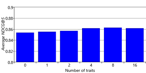
You may be wondering why we see an increase in average NDCG when there is no increase in prediction accuracy. The answer is that NDCG is a more sensitive metric because it makes use of the original ground truth star ratings, rather than these ratings converted into likes/dislikes. This sensitivity suggests that we would benefit by training our model on the full range of star ratings rather than just on a binary like or dislike. In the next section, we will explore what model changes we need to make to achieve this.
Discounted Cumulative GainA metric for a list of recommendations that is defined as the sum of scores for each individual recommendation, weighted by a discount function that depends on the position of that recommendation in the list. The discount function is selected to give higher weights to recommendations at the start of the list and lower weights towards the end. Therefore, the DCG is higher when good recommendations are put at the start of the list than when the list is reordered to put them at the end. See Figure 5.16 for a visual example of calculating DCG.
Normalized Discounted Cumulative GainA scaled version of the Discounted Cumulative Gain, where the scaling makes the maximum possible value equal to 1. This scaling is achieved by dividing by the actual DCG by the maximum possible DCG. See Figure 5.16 and Figure 5.17 for visual examples of calculating a DCG and a maximum possible DCG.