-

Want a paper copy?
You can now buy the book!
All royalties go to the Cystic Fibrosis Trust.Spotted an error? Have comments?
Let us know!Get hands on with source code for the book.
6.4 Modelling with gates

A gate allows part of a factor graph to be turned on or off.
In the previous section, we saw how to compare alternative processes by manually inferring the posterior distribution over a random variable that selects between them. What we will now see is how to do the same calculation by defining an appropriate model and performing inference within that model. To do this, we need a new modelling structure that allows alternatives to be represented within a model. The modelling structure that we can use to do this is called a gate, as described in Minka and Winn [2009].
A gate encloses part of a factor graph and switches it on or off depending on the state of a random variable called the selector variable. The gate is on when the selector variable has a particular value, called the key, and off for all other values. An example gate is shown in the factor graph of Figure 6.11. The gate is shown as a dashed rectangle with the key value (true) in the top left corner. The selector variable selector has an edge connecting it to the gate – the arrow on the edge shows that the gate is considered to be a child of the selector variable. When selector equals true, the gate is on and so x has a Bernoulli(0.2) distribution. Otherwise, the gate is off and x has a uniform distribution, since it is not connected to any factors.
|
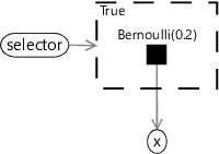
When writing the joint distribution for a factor graph with a gate, all terms relating to the part of the graph inside the gate need to be switched on or off according to whether the selector variable takes the key value or not. Such terms can be turned off by raising them to the power zero and left turned on by raising to the power one. For example, the joint distribution for Figure 6.11 is
where the function equals one if the expression in brackets is true and zero otherwise. If selector is not true the term will be raised to the power zero, making the term equal to one – equivalent to removing it from the product (i.e. turning it off).
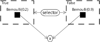
When using gates inside a model, it is common to have a gate for each value of the selector variable. In this case, the resulting set of gates is called a gate block. Because the selector variable can only have one value, only one gate in a gate block can be on at once. An example gate block is shown in the factor graph of Figure 6.12. In this example, the selector variable is binary and so there are two gates in the gate block, one with the key value true and one with the key value false. It is also possible to have selector variables with any number of values, leading to gate blocks containing the corresponding number of gates.
|
The joint probability distribution for this factor graph is
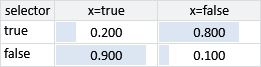
Looking at this joint probability, you might be able to spot that the gate block between selector and x represents a conditional probability table, like so:
As another example, we can represent the conditional probability table for the skin test (Figure 6.1) using gates like this:
|
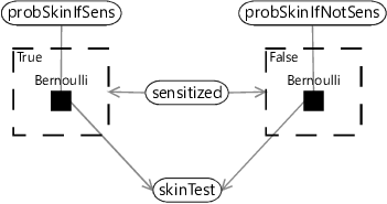
Representing this conditional probability table using a gate block is less compact than using a Table factor (as we did in Figure 6.1) but has the advantage of making the relationship between the parent variable and child variable more clear and precise. When a variable has multiple parents, using a gate block to represent a conditional probability table can also lead to more accurate or more efficient inference.
Using gates for model selection
Representing a conditional probability table is just the start of what can be achieved using gates. For example, they can also be used to do model selection. To see how, let’s return to our model selection problem from the previous section. Remember that we wanted to select between a ‘has effect’ model and a ‘no effect’ model, by inferring the posterior distribution of a random variable called model. Using gates, we can represent this model selection problem as a single large factor graph, using a gate block where the selector variable is model. We then place the entire ‘no effect’ model inside a gate whose key value is NoEffect and the entire ‘has effect’ model inside the other gate of the block whose key value is HasEffect. The observed variables are left outside of both gates because they are common to both models and so are always on. The result is the factor graph in Figure 6.14.
|
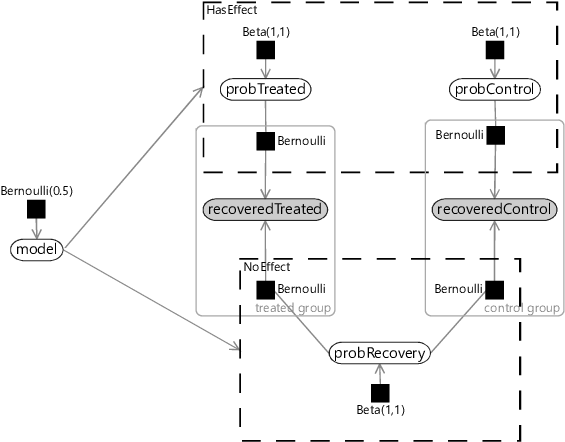
This factor graph may look a bit scary, but it can be interpreted in pieces. The top gate contains exactly the model from Figure 6.10 with the observed variables outside the gate. The bottom gate contains exactly the model from Figure 6.9 drawn upside down and sharing the same observed variables. Finally we have one new variable which is our model variable used to do model selection.
Given this factor graph, we just need to run expectation propagation to infer the posterior distribution over model. Right? Well, almost – it turns out that first we need to make some extensions to expectation propagation to be able to handle gates. The good news is that these modifications allow expectation propagation to be applied to any factor graph containing gates.
Expectation propagation in factor graphs with gates
In this optional section, we see how to use expectation propagation to compute model evidence and then how to extend expectation propagation to work on graphs containing gates. If you want to focus on modelling, feel free to skip this section.
To run expectation propagation in a factor graph which contains gates, we first need to be able to compute the model evidence for a factor graph without gates. It turns out that we can compute an approximation to the model evidence by using existing EP messages to compute evidence contributions for each variable and factor individually, and then multiplying them together. For example, the evidence contribution for a variable x is given by:
This equation states that to compute the evidence for a variable x, first take the product of all incoming messages on edges connected to the variable, then sum the result over the values that x can take (this is what the notation means). Because of this sum the result is a single number rather than a distribution – this number is the local contribution to the model evidence.
The evidence contribution for a factor f connected to multiple variables Y is given by:
In this equation, the notation means the sum over all joint configurations of the connected variables Y.
We can use equations (6.14) and (6.15) to calculate evidence contributions for every variable and factor in the factor graph. The product of all these contributions gives the EP approximation to the model evidence. For a model M, this gives:
In equation (6.16), the first term means the product of the evidence contributions from every variable in model M and the second term means the product of evidence contributions from every factor in model M.
Adding in gates
If we now turn to factor graphs which contains gates, there is a new kind of evidence contribution that comes from any edge that crosses over a gate boundary. If such an edge connects a variable x to a factor f, then the evidence contribution is:
In other words, we take the product of the two messages passing in each direction over the edge and then sum the result over the values of the variable x.
The advantage of computing evidence contributions locally on parts of the factor graph is that, as well as computing evidence for the model as a whole, we can also compute evidence for any particular gate. The evidence for a gate is the product of the evidence contributions for all variables and factors inside the gate, along with the contributions from any edges crossing the gate boundary. For a gate g, this product is given by:
If there are no edges crossing the gate boundary – in other words, the gate contains an entire model disconnected from the rest of the graph – then this equation reduces to the model evidence equation (6.16) above, and so gives the evidence for the contained model.
Given these evidence contributions, we can now define an extended version of expectation propagation which works for factor graphs that contain gates. The algorithm requires that gates only occur in gate blocks and that any variable connecting to a factor in one gate of a gate block, also connects to factors in all other gates of the gate block. This ‘gate balancing’ can be achieved by connecting the variable to uniform factors in any gate where it does not already connect to a factor. We need this gate balancing because messages will be defined as going to or from gate blocks, rather than to or from individual gates.
When sending messages from a factor f inside a gate g to a variable x outside the gate, we will need to weight the message appropriately, using a weight defined as:
where the notation indicates that we are evaluating the probability of the gate’s key value under the distribution given by the message from the selector variable. Using these weights, we can define our extended expectation propagation algorithm as shown in Algorithm 6.1.
- Selector variable to gate block: the product of all messages received on the other edges connected to the selector variable;
- Gate block to selector variable: a distribution over the selector variable where the probability of each value is proportional to the evidence for the gate with that key value;
- Factors in gate block to variable outside gate block: Compute weighted sum of messages from the factor in each gate using weights given by (6.19). Multiply by the context message (the message coming from the variable to the gate block). Project into the desired distribution type using moment matching. Divide out the context message.
- All other messages: the normal EP message (defined in Algorithm 3.1);
The full derivation of this algorithm is given in Minka and Winn [2009], along with some additional details that we have omitted here (such as how to handle nested gates).
Now that we have a general-purpose inference algorithm for gated graphs, we can use it to do Bayesian model selection and to infer posterior distributions over variables of interest, both at the same time! For example, recall the example trial from section 6.3. In this trial, 13 out of 20 people in the treated group recovered compared to 8 out of 20 in the control group. Attaching this data to the gated factor graph of Figure 6.14, we can apply expectation propagation to compute posteriors over the model selection variable model and also over other variables such as probTreated and probControl. The results are shown in Figure 6.15.
 Excel
Excel CSV
CSV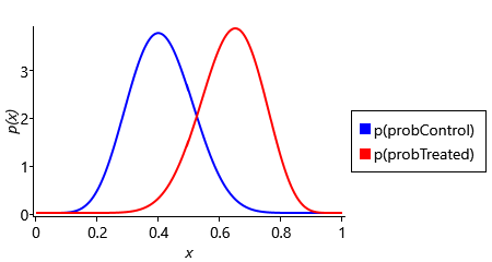
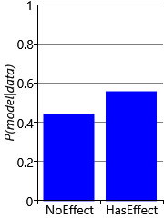
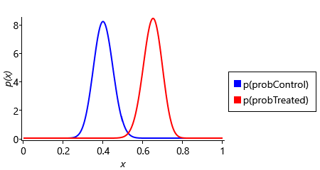
Figure 6.15 shows that the posterior distribution over model puts slightly higher probability on the ‘has effect’ model than on the ’no effect’ model. The exact values are 0.5555 for model=HasEffect and 0.4445 for model=NoEffect. The ratio of these probabilities is the Bayes factor, which in this case is 1.25. This is the same value that we computed manually in section 6.3, showing that for this model the expectation propagation posterior is exact. The posterior distributions over probControl and probTreated give an indication of why the Bayes factor is so small. The plots show that there is a lot of overlap between the two distributions, meaning that is possible that both probabilities are the same value, in other words, that the ’no effect’ model applies.
Let’s see what happens when we increase the size of the trial, but leave the proportions of people who recovered the same in each group. For a trial of three times the size, this would see 39 out of 60 recovered in the treated group compared to 24 out of 60 in the control group. Plugging this new data into our model, gives the results shown in Figure 6.16.
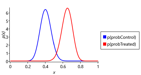
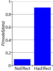
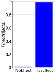
Figure 6.16 shows that, after tripling the size of the trial, the ‘has effect’ model has a much higher probability of 0.904, giving a Bayes factor of 9.41. Since this factor lies in the range 3-20, the outcome of this trial can now be considered positive evidence in favour of the ‘has effect’ model. The posterior distributions over probControl and probTreated shows why the Bayes factor is now much larger: the two curves have much less overlap, meaning that the chances of the two probabilities being the same is much reduced. We can take this further and increase the trial size again so that it is five times the size of the original trial. In this larger trial, 65 out of 100 recovered in the treated group compared to 40 out of 100 in the control group, giving the results shown in Figure 6.17.
In Figure 6.17, the posterior distributions over probControl and probTreated hardly overlap at all. As a result, the ‘has effect’ model now has a probability of 0.989, giving a Bayes factor of 92.4. Since this factor lies in the range 20-150, the outcome of this trial can now be considered strong evidence in favour of the ‘has effect’ model. These results show the importance of running a large enough clinical trial if you want to prove the effectiveness of your new drug!
Now that we understand how gates can be used to model alternatives in our randomised controlled trial model, we are ready to use gates to model alternative sensitization classes in our allergy model, as we will see in the next section.
gateA container in a factor graph that allows the contained piece of the graph to be turned on or off, according to the value of another random variable in the graph (known as the selector variable). Gates can be used to create alternatives within a model and also to do model selection. More details of gates can be found in Minka and Winn [2009] or in the expanded version Minka and Winn [2008].
selector variableA random variable that controls whether a gate is on or off. The gate will specify a particular key value – when the selector variable has that value then the gate is on; for any other value it is off. For an example of a selector variable, see Figure 6.11.
gate blockA set of gates each with a different key value corresponding to the possible values of a selector variable. For any value of the selector variable, one gate in the gate block will be on and all the other gates will be off. An example gate block is shown in the factor graph of Figure 6.12.
[Minka and Winn, 2009] Minka, T. and Winn, J. (2009). Gates. In Advances in Neural Information Processing Systems 21.