6.5 Discovering sensitization classes
Now that we have gates in our modelling toolbox, we can extend our allergy model so that different children can have different patterns of allergy gain and loss. As you may recall from section 6.2, the model change that we want to make is to encode this modified assumption:
- The probabilities relating to initially having, gaining or retaining sensitization to a particular allergen are the same for all children
in each sensitization class.
This assumption requires that each child belongs to some sensitization class, but we do not know which class each child belongs to. We can represent this unknown class membership using a sensClass random variable for each child, which takes a value in depending on whether the child is in class 0, class 1 and so on. Because this variable can take more than two values, we cannot use a Bernoulli distribution to represent its uncertain value. Instead we need a discrete distribution, which is a generalisation of a Bernoulli distribution to variables with more than two values.
Our aim is to do unsupervised learning of this sensClass variable – in other words, we want to learn which class each child is in, even though we have no idea what the classes are and we have no labelled examples of which child is in which class. Grouping data items together using unsupervised learning is sometimes called clustering. The term clustering can be misleading, because it suggests that data items naturally sit together in unique clusters and we just need to use machine learning to reveal these clusters. Instead, data items can usually be grouped together in many different ways, and we choose a particular kind of grouping to meet the needs of our application. For example, in this asthma project, we want to group together children that have similar patterns of allergic sensitization. But for another project, we could group those same children in a different way, such as by their genetics, by their physiology and so on. For this reason, we will avoid using the terms ‘clustering’ and ‘clusters’ and use the more precise term ‘sensitization class’.
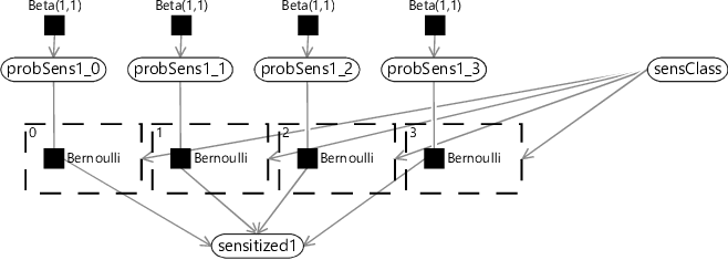
Each sensitization class needs to have its own patterns of gaining and losing allergic sensitizations, with the corresponding probabilities for gaining and losing sensitizations at each time point. For example, each class should have its own value of probSens1 which gives the probability of sensitization at age 1 for children in that particular sensitization class. To achieve this in our model, we need the sensitization state at age 1 (sensitized1) to be connected to the appropriate probSens1 corresponding to the sensitization class of the child. We can achieve this by replicating the connecting Bernoulli factor for each sensitization class, and then using a gate block to ensure that only one of these factors is turned on, as shown in Figure 6.18.
In Figure 6.18, we have assumed that there are four sensitization classes and duplicated probSens1 into separate probabilities for each class (probSens1_0, probSens1_1 …). There is a gate for each class, keyed by the number of the class (0,1,2 or 3). Because each key is different, any value of sensClass leads to one gate being on and all the other gates being off. In this way, the value of sensClass determines which of the four initial sensitization probabilities to use.
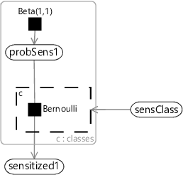
The factor graph of Figure 6.18 is quite cluttered because of the repeated factors and variables for each sensitization class. We can represent the same model more compactly if we introduce a plate across the sensitization classes and put the repeated elements inside the plate, as shown in Figure 6.19.
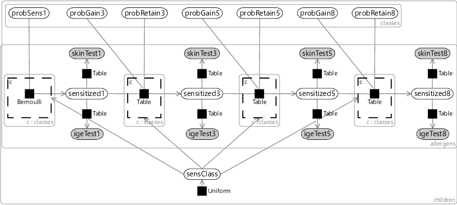
Using the compact notation of Figure 6.19, we can modify our allergy model of Figure 6.5 to have different probabilities for each sensitization class. We take all our probability variables probSens1, probGain3 and so on, and duplicate them across classes using a plate. We then place each factor in the Markov chain inside a gate and plate, where the gates are all connected to a sensClass selector variable. Finally, we choose a uniform prior over sensClass, giving the factor graph of Figure 6.20.
Testing the model with two classes
To test out our model in its simplest form, we can set the number of sensitization classes to two. With just two classes, we would expect the model to divide the children into a group which have no sensitizations and a second group that contains those children with sensitizations. However, when we run expectation propagation in the model, we get an unexpected result. The posterior distributions over the sensitization class are all uniform, for every child! In addition, when we look at the learned probabilities of gaining/retaining sensitizations, they are also all the same for each class – and look just like the one-class probabilities shown in Figure 6.7. What has happened here?
The issue is that our model defines every sensitization class in exactly the same way – each class has the same set of variables which all have exactly the same priors. We could reorder the sensitization classes in any order and the model would be unchanged. This self-similarity is a symmetry of the model, very similar to the symmetry we encountered in section 5.3 in the previous chapter. During inference, this symmetry causes problems because the posterior distributions will not favour any particular ordering of classes and so will end up giving an average of all classes – in other words, the same results as the one-class model. Not helpful!
As in the previous chapter, we need to apply some kind of symmetry breaking to get useful inference results. In this case, we can break symmetry by providing initial messages to our model, such that the messages differ from class to class. A simple approach is to provide an initial message into each sensClass variable which is a point mass at a randomly selected value. The effect of these initial messages is to randomly assign children to sensitization classes for the first iteration of expectation propagation. This randomization affects the messages going to the class-specific variables (such as probSens1) in the first iteration, which in turn means that the messages to each sensClass variable are non-uniform in the next iteration and so on. The end result is that the class-specific variables eventually converge to describe different underlying sensitization classes and the sensClass variables converge to assign children to these different classes.
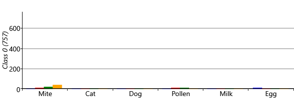
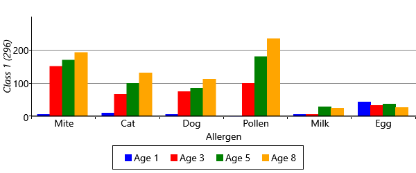
With symmetry breaking in place, we can now run inference successfully in a two-class model. We can visualize the results using a chart like Figure 6.8 for each class. To do this, we assign each child to the sensitization class with the highest posterior probability, giving the plots of Figure 6.21 for the two classes. The figure shows that the model has picked up on a large class of 757 children who have virtually no sensitizations and a smaller class of 296 children who do have sensitizations. In other words, the two-class model has behaved as expected and separated out the children who have sensitizations from those who do not.
Exploring more sensitization classes
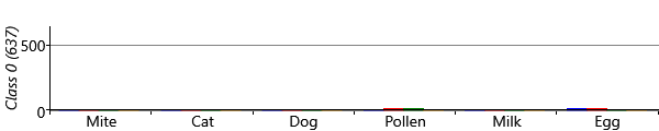
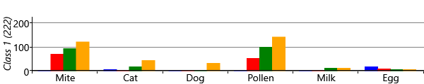
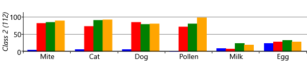
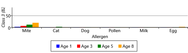
The results for two classes provide a useful sanity check that the model is doing something reasonable. However, we are really interested in what happens when we have more than two classes, since we hope additional classes would uncover new patterns of sensitization. Let’s consider running the model with five possible classes. We say five ‘possible’ classes, because there is no guarantee that all classes will be used. That is, it is possible to run the inference algorithm and find that there are classes with no children assigned to them. With our model and data set, we find that it is common when running with five classes, that only four of them are actually in use. Effectively the number of classes in the model defines a maximum on the number of classes found – which allows for the number of classes itself to be learned. Different random initialisations give slightly different sensitization classes, but often these contain very similar looking classes. Figure 6.22 shows some typical results for the four classes found when up to five were allowed in the model.
As you can see from Figure 6.22, model has divided the children with sensitizations into three separate classes. The largest of these, Class 1, contains 222 children who predominantly have mite and pollen allergies, but have few other allergies. In contrast, Class 2 contains 112 children who have allergies to cat and dog as well as mite and pollen. This class also contains those children who have milk and egg allergies. It is also worth noting that the children in this class acquire their allergies early in life – in most cases by age 3. The final class, Class 3 is relatively small and contains 82 children who predominantly have mite allergies.
These results demonstrate the strength of unsupervised learning – it can discover patterns in the data that you did not expect in advance. Here we have uncovered three different patterns of sensitization that we were not previously aware of. The next question to ask is “how does this new knowledge help our understanding of asthma?”. To answer this question, we can see if there is any link between which sensitization class a child belongs to and whether they went on to develop asthma.
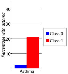
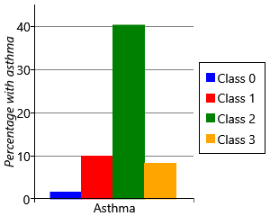
For each child, our data set contains a measurement of whether they had developed asthma by age 8. For each of the two class and four class models, we can use these measurements to plot the percentage of children in each sensitization class that went on to develop asthma. The results are shown in Figure 6.23.
Let’s start by looking at plots for the two class model. As we might expect, the percentage of children with asthma is higher in the class with sensitizations (class 1), than the class without sensitizations (class 0). Indeed, the presence of allergic sensitizations is used as a predictor of developing asthma. But when we look at the results for the four class model, we see a very interesting result – whilst all the classes with sensitizations show an increased percentage of children developing asthma, class 2 shows a much higher percentage than any other class. It seems that children who have the broad set of allergies characterised by class 2 are more than four times as likely to develop asthma than children who have other patterns of allergies! This is a very exciting and clinically useful result. Indeed, when we looked further we found that this pattern of allergies also led to an increased chance of severe asthma with an associated increased risk of hospital admission [Simpson et al., 2010]. Being able to detect such severe asthma early in life, could help prevent such life-threatening episodes from occurring.
In summary, in this chapter, we have seen how unsupervised learning discovered new patterns of allergic sensitization in our data set. In this case, these patterns have led to a new understanding of childhood asthma with the potential of significant clinical impact. Although, in general, unsupervised learning can be more challenging than supervised learning, the value of the new understanding that it delivers frequently justifies the extra effort involved.
Review of concepts introduced on this page
discrete distributionA probability distribution over a many-valued random variable which assigns a probability to each possible value. The parameters of the distribution are these probabilities, constrained to add up to 1 across all possible values. This distribution is also known as a categorical distribution.
An example of a discrete distribution is the outcome of rolling a fair dice, which can be written as Discrete The Bernoulli distribution is actually a special case of a discrete distribution for when there are only two possible values.
clusteringA form of unsupervised learning where data items are automatically collected into a number of groups, which are known as clusters. Each cluster is then assumed to contain items which are in some way similar.
References
[Simpson et al., 2010] Simpson, A., Tan, V., Winn, J., Svensen, M., Bishop, C., Heckerman, D., Buchan, I., and Custovic, A. (2010). Beyond atopy: Multiple patterns of sensitization in relation to asthma in a birth cohort study. American Journal of Respiratory and Critical Care Medicine, 181:1200–1206.

 Excel
Excel CSV
CSV