-

Want a paper copy?
You can now buy the book!
All royalties go to the Cystic Fibrosis Trust.Spotted an error? Have comments?
Let us know!Get hands on with source code for the book.
3.2 Inferring the players’ skills
So far we have assumed that we know the skills of Jill and Fred, and we have used these skills to compute the probability that each of the players would be the winner. In practice, we have to reason backwards: we observe who wins the game and need to use this information to learn about the skill values of the players. We therefore turn to the problem of learning player skills.

In any game, seeing who wins and who loses tells us about the skill of the players.
Given the outcome of a game it would seem reasonable to increase the skill value for the winner and decrease the skill value for the loser. What is less clear, however, is how big an adjustment we should make. Intuitively we can reason as follows. Suppose that Jill is the winner of the game. If Jill’s skill is significantly higher than Fred’s, then it is unsurprising that Jill should be the winner, and so the change in skill values should be relatively small. If the skills are similar then a larger change would be justified. However, if Jill’s skill is significantly less than Fred’s then the game outcome is very surprising. The outcome suggests that our current assessments of the skill values are not very accurate, and therefore that we should make a much larger adjustment in skill values. Put concisely, the degree of surprise gives an indication of how big a change in skill values should be made. We will see that performing inference in a suitable model automatically gives this kind of behaviour.
Modelling skills
We have already noted that skill is an uncertain quantity, and should therefore be included in the model as a random variable. We need to define a suitable prior distribution for this variable. This distribution captures our prior knowledge about a player’s skill before they have played this particular game. For a new player, this distribution would need to be broad and cover the full range of skills that the player might have. For a more established player, we may already have a good idea of their skill and so the distribution would be narrower. Because skill is a continuous variable, we can once again use a Gaussian distribution to define this prior. This represents a modification to our first modelling assumption, which becomes:
- Each player has a skill value, represented by a continuous variable with a Gaussian prior distribution.
Let us return to our game of Halo between Jill and Fred. So far we have assumed that the skill values for Jill and Fred are known and have values of 15 and 12.5 respectively. For the remainder of the chapter we shall instead assume that the skills for Jill and Fred are not known, but have uncertainty represented by a Gaussian distribution. For Jill, we will now assume a mean skill of 120 with a standard deviation of 40 – this would typically arise if Jill is a relatively new player and so there is a lot of uncertainty in her skill . For Fred, we will now assume a mean skill of 100 with a standard deviation of 5 which would be reasonable if Fred is a more established player whose skill is more precisely known. We must therefore extend our model by introducing two more uncertain variables Jskill and Fskill: the skills of Jill and Fred. Each of these variables will have its own Gaussian distribution and therefore its own factor in the factor graph. The factor graph for our extended model is shown in Figure 3.10.
|
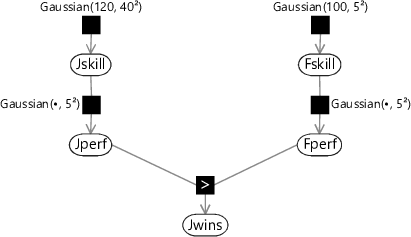
The model in Figure 3.10 was developed by Herbrich et al. [2007] who called it the TrueSkill model. As a reminder, the assumptions that are encoded in the model are all shown together in Figure 3.11.
- Each player has a skill value, represented by a continuous variable with a broad Gaussian distribution.
- Each player has a performance value for each game, which is independent from game to game and has an average value is equal to the skill of that player. The variation in performance, which is the same for all players, is symmetrically distributed around the mean value and is more likely to be close to the mean than to be far from the mean.
- The player with the higher performance value wins the game.
Having stated our modelling assumptions explicitly, it is worth taking a moment to review them. Assumptions0 3.1 says that a player’s ability at a particular type of game can be expressed as a single continuous variable. This seems reasonable for most situations, but we could imagine a more complex description of a player’s abilities which, for example, distinguishes between their skill in attack and their skill at defence. This might be important in team games (discussed later) where a strong team may require a balance of players with strong attack skills and those with good defensive skills. We also assumed a Gaussian prior for the skill variable. This is the simplest probabilistic model we could have for a continuous skill variable, and it brings some nice analytical and engineering properties. However, if we looked at the skills of a large population of players we might find a rather non-Gaussian distribution of skills, for example, new players may often have low skill but, if they have played a similar game before, may occasionally have a high skill.
Similarly, Assumptions0 3.2 considers a single performance variable and again assumes it has a Gaussian distribution. It might well be the case that players can sometimes have a seriously ‘off’ day when their performance is way below their skill value, while it would be very unlikely for a player to perform dramatically higher than their skill value. This suggests that the performance distribution might be non-symmetrical. Another aspect that could be improved is the assumption that the variance is the same for all players – it is likely that some players are more consistent than others and so would have correspondingly lower variance.
Finally, Assumptions0 3.3 says that the game outcome is determined purely by the performance values. If we had introduced multiple variables to characterize the skill of a player, there would presumably each have a corresponding performance variable (such as how the player performed in attack or defence), and we would need to define how these would be combined in order to determine the outcome of a game.
Inference in the TrueSkill model
Once a game has been played, we aim to use the outcome of the game to infer the updated skill distribution for the players. This involves solving a probabilistic inference problem to calculate the posterior distribution of each player’s skill, taking account of the new information provided by the result of the game. Although the prior distribution is Gaussian, it turns out that the corresponding posterior distribution is not Gaussian. The following section shows how to compute the posterior distribution for the skill and why it is not Gaussian – feel free to skip it or return to it later if you prefer.
In this optional section, we see how to do exact inference in the model as defined so far, and then we see why exact inference is not useable in practice. If you want to focus on modelling, feel free to skip this section.
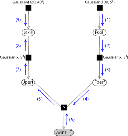
Now that we have the factor graph describing our model, we can set the variable Jwins according to the observed game outcome and run inference in order to compute the marginal posterior distributions of the skill variables Jskill and Fskill. The graph has a tree structure (there are no loops) and so we have already seen in Chapter 2 that we can solve this problem using belief propagation.
Consider the evaluation of the posterior distribution for Jskill in the case where Jill won the game (Jwins is true). Using the belief propagation algorithm we have to evaluate the messages shown in Figure 3.12.
(5) (9) (8) (1) (2) (7) (6) (3) (4)
|
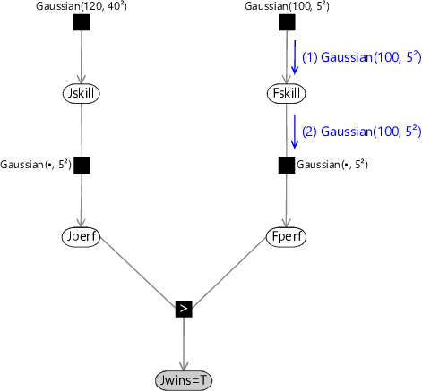
Message (1) is just given by the Gaussian factor itself. Similarly, message (2) is just the product of all incoming messages on other edges of the Fskill node, and since there is only one incoming message this is just copied to the output message. These first two messages are summarized in Figure 3.13.
(1) Gaussian(100, 5²)(2) Gaussian(100, 5²)
|
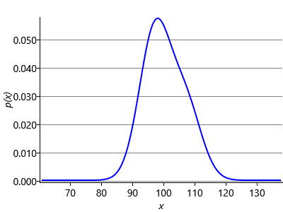
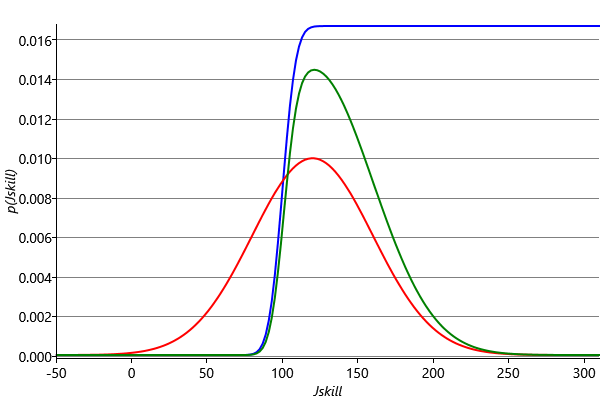
Next we have to compute message (3) in Figure 3.12. The belief propagation algorithm tells us to multiply the incoming message (2) by the Gaussian factor and then sum over the variable Fskill. In this case the summation becomes an integration because Fskill is a continuous variable. We can gain some insight into this step by once again considering a generative viewpoint based on sampling. Imagine that we draw samples from the Gaussian distribution over Fskill. Each sample is a specific value of Fskill and forms the mean of a Gaussian distribution over Fperf. In Figure 3.14a we consider three samples of Fskill and plot the corresponding distributions over Fperf. To compute the desired outgoing message we then average these samples, giving the result shown in Figure 3.14b. This represents an approximation to the marginalization over Fskill, and would become exact if we considered an infinite number of samples instead of just three.
 Excel
Excel CSV
CSV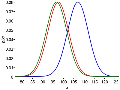
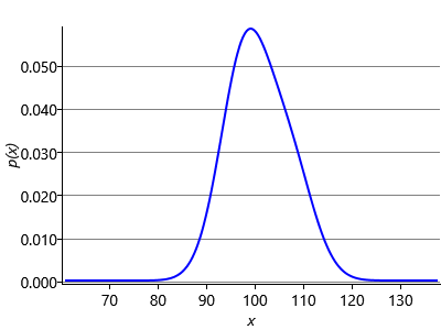
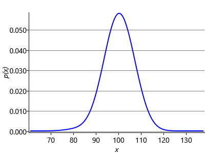
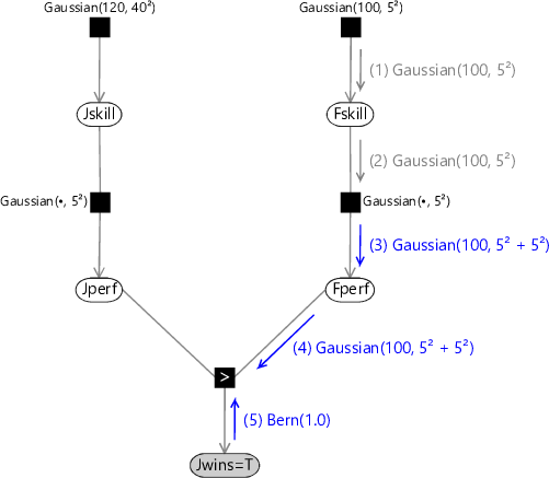
The sampling approximation becomes more accurate as we increase the number of samples, as shown in Figure 3.14c and Figure 3.14d. In this final figure the resulting distribution looks almost Gaussian. This is not a coincidence, and in fact the calculation of the outgoing message can be worked out exactly (see Equation (2.115) in Bishop [2006]) with the result that the outgoing message is also a Gaussian whose mean is the mean of the distribution of Fskill and whose variance is the sum of the variances of Fskill and Fperf: . This process of ‘smearing’ out one Gaussian using the other Gaussian is an example of a mathematical operation called convolution. Message (4) is just a copy of message (3) as there is only one incoming message to the Fperf node. Since we observe that Jwins is true, message (5) is a Bernoulli point mass at the value true. These three messages are illustrated in Figure 3.15.
(1) Gaussian(100, 5²)(2) Gaussian(100, 5²)(3) Gaussian(100, 5² + 5²)(4) Gaussian(100, 5² + 5²)(5) Bern(1.0)
|
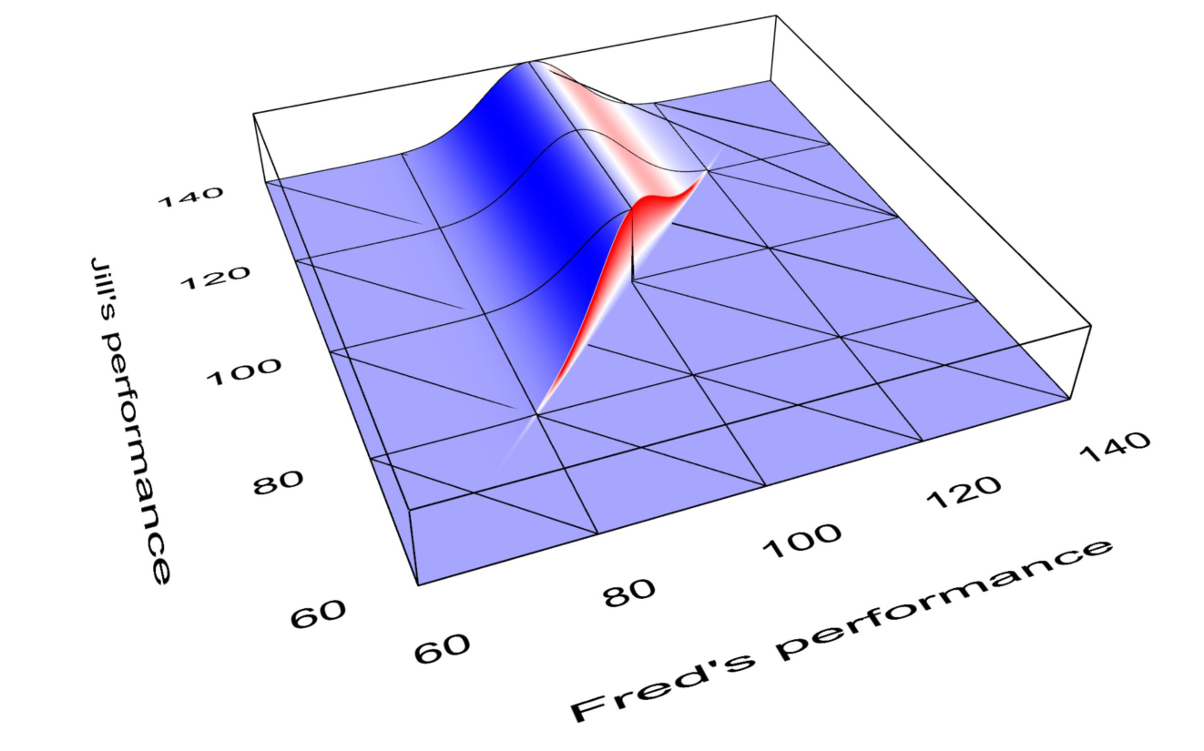
Now let’s turn to computing message (6). The observation that Jill wins (Jwins=true) applies a constraint that the performance of Jill must be higher than that of Fred, so . This constraint is applied when we multiply in the GreaterThan factor with the value of Jwins set to true. Figure 3.16 shows the effect of multiplying in this constraint to the Gaussian message coming from Fperf. In the figure, the product is always zero below the diagonal line – in other words, where . This area is set to zero because it corresponds to Fred winning, which has zero probability because it contradicts our observation that Jill won. So we end up with a Gaussian ’bump’ truncated at the diagonal.
To compute message (6), we have to integrate the product in Figure 3.16 over Fperf, to give a message which is a function of Jperf. You can visualize this message by imagining looking the truncated Gaussian bump from the direction of the axis for Jill’s performance and summing over what can be seen from each point. The resulting message is zero below about 80, and then curves up to near one at about 120 and then remains there up to infinity, as shown in Figure 3.17.
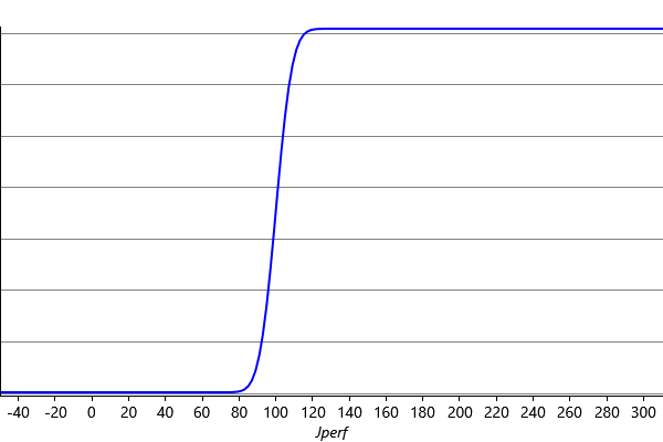
The reader should take a moment to confirm that shape of this function is what would be expected from integrating Figure 3.16 over the variable Fperf. Mathematically, for each value of Jperf a truncated Gaussian distribution is being integrated, this is equivalent to the evaluation of the cumulative Gaussian that we introduced back in equation (3.10), and so this message can be evaluated analytically (indeed, this is how Figure 3.17 was plotted).
For another interpretation of the shape of this message, suppose we knew that Fperf was exactly 100. Given that Jill won, this tells us that Jill’s performance Jperf must be some number greater than 100. This would mean a message in the form of a step, with the value zero below 100 and some positive constant above it. Since, we don’t know that Fperf is exactly 100, but only know that it is likely to be near 100, this smears out the step into the smooth function of Figure 3.17.
Because message (6) continues up to infinity, it forms what we call an improper distribution, which is a distribution whose area cannot be normalized to sum to one. In belief propagation, messages are allowed to be improper, provided that they do not cause posterior marginal distributions to become improper. For example, in this case, the improper message will be multiplied by a proper normalized message, giving a posterior which can be normalized and so is proper.
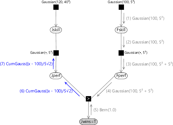
Message (7) is just a copy of message (6) since there is only one incoming message to the Jperf node. These messages are illustrated in Figure 3.18
(5) Bern(1.0)(1) Gaussian(100, 5²)(2) Gaussian(100, 5²)(6) CumGauss((x - 100)/5√2) (3) Gaussian(100, 5² + 5²)(4) Gaussian(100, 5² + 5²)(7) CumGauss((x - 100)/5√2)
|
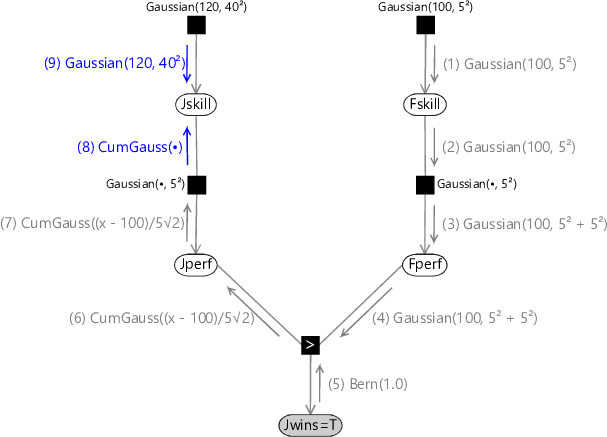
Message (8) is found by multiplying the Gaussian factor describing the performance variability by the incoming message (7) and then integrating over Jperf. This again is a convolution, and has an exact solution again in the form of a cumulative Gaussian. Effectively it is a blurred version of the incoming cumulative Gaussian message which has been smeared out by the variance of the Gaussian performance factor. Finally, message (9) is the Gaussian distribution for the skill prior. These messages are summarized in Figure 3.19.
(5) Bern(1.0)(8) CumGauss(•)(1) Gaussian(100, 5²)(2) Gaussian(100, 5²)(7) CumGauss((x - 100)/5√2) (6) CumGauss((x - 100)/5√2) (3) Gaussian(100, 5² + 5²)(4) Gaussian(100, 5² + 5²)(9) Gaussian(120, 40²)
|
To obtain the marginal distribution of Jskill we then multiply messages (8) and (9). Because this is the product of a Gaussian and a cumulative Gaussian the result is a bump-like distribution which is not symmetrical, and therefore is not a Gaussian. These messages, and the resulting marginal distribution for Jskill, are shown in Figure 3.20.
We seem to have solved the problem of finding the posterior distribution for Jskill. We can also pass messages in the opposite direction around the graph to obtain the corresponding posterior distribution for Fskill. These posterior distributions can be expressed exactly as the product of a Gaussian and a cumulative Gaussian and so require four parameters to describe them, where the two additional parameters come from the cumulative Gaussian.
A problem with using exact inference
We now have a way to compute posterior distributions over the skills of our players. The problem is that these posterior distributions are not Gaussian. Instead, they have a more complex form of distribution which requires four numbers to express, instead of two for a Gaussian. This difference causes a major problem if we imagine, say, Jill going on to play another game with a new player. Before the game with Fred, our uncertainty in the value of Jskill was expressed as a Gaussian distribution, which has two parameters (the mean and the variance). After she has played against Fred the corresponding posterior distribution is expressed as a more complex distribution with four parameters. Now suppose that Jill plays another game of Halo against Alice. We can again represent this by a factor graph similar to Figure 3.10, except that the factor describing our current uncertainty in Jskill is now the posterior distribution resulting from the game against Fred. When we run inference in this new graph, to take account of the outcome of the game against Alice, the new posterior marginal will be an even more complex distribution which requires six parameters (to be specific, a product of a Gaussian and two different cumulative Gaussians). Each time Jill plays a game of Halo the distribution over her skill value requires two additional parameters to represent it, and the number of parameters continues to grow as she plays more and more games. This is not a practical approach to use in an engineering application.
Notice that this problem would not arise if the posterior distribution for the variable of interest had the same form as the prior distribution. In some probabilistic models we are able to choose a form of prior distribution, known as a conjugate prior, such that the posterior ends up having the same form as the prior. Take a look at Panel 3.2 to learn more about conjugate distributions.
From a message-passing perspective, conjugacy means that the product of all messages arriving at a variable node has the same form as the prior message. This general means that all the incoming messages have the same form as the prior message. In our model, the upwards message from the GreaterThan factor is not Gaussian, and so nor is the one up to the Jskill variable. This means that the prior Gaussian distribution is not a conjugate distribution for Jskill.
Without conjugacy, it is necessary to introduce some form of approximation, to allow the posterior of Jskill to remain Gaussian. In the next section, we will describe a powerful algorithm that extends belief propagation by allowing messages to be approximated even when they are not conjugate. This algorithm will not only solve the inference problem with this model, but turns out to be applicable to a wide variety of other probabilistic models as well - including every single model in this book!
convolutionThe convolution of a function with a function measures the overlap between and a version of which is translated by an amount . It is expressed as a function of . For more information see Wikipedia.
improper distributionA distribution whose area does not sum to one.
conjugate distributionFor a given likelihood function, a prior distribution is said to be conjugate if the corresponding posterior distribution has the same functional form as the prior.
The following exercises will help embed the concepts you have learned in this section. It may help to refer back to the text or to the concept summary below.
- Reproduce Figure 3.14 by plotting the average of Gaussian distributions each with standard deviation is 5 and with mean is given by a sample from a . Do this for , and .
- Referring to Panel 3.2, use Bayes’ theorem to compute the posterior distribution over (the probability of clicking on the buy button) given that people do click on the button but people do not click on it. Assume a prior distribution. Notice that this is a conjugate prior and so the posterior distribution is also a beta distribution.
- [Advanced] Show that the convolution of two Gaussian distributions is also a Gaussian distribution whose variance is the sum of the variances of the two original distributions. Section 2.3.3 in Bishop [2006] should help.
[Herbrich et al., 2007] Herbrich, R., Minka, T., and Graepel, T. (2007). TrueSkill(TM): A Bayesian Skill Rating System. In Advances in Neural Information Processing Systems 20, pages 569–576. MIT Press.
[Bishop, 2006] Bishop, C. M. (2006). Pattern Recognition and Machine Learning. Springer.