-

Want a paper copy?
You can now buy the book!
All royalties go to the Cystic Fibrosis Trust.Spotted an error? Have comments?
Let us know!Get hands on with source code for the book.
3.4 Extensions to the core model
So far, we have constructed a probabilistic model of a game played between two players which results in a win for one of the players. To handle the variety of games needed by Xbox Live, we need to extend our model to deal with a number of additional complexities. In particular, real games can end in draws, can involve more than two players, and can be played between teams of people. We will now show how our initial model can be extended to take account of these complexities. This flexibility nicely illustrates the power of a model-based approach to machine learning.
Specifically, we need to extend our model so that it can:
- update the skills when the outcome is a draw;
- update the skills of individual team members, for team games;
- apply to games with more than two players.
A model-based approach allows such extensions to be incorporated in a transparent way, giving rise to a solution which can handle all of the above complexities – whilst remaining both understandable and maintainable.
What if a game can end in a draw?
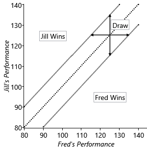
In our current model, the player with the higher performance value on a particular game is the winner of that game. For games which can also end in a draw, we can modify this assumption by introducing the concept of a draw margin, such that a player is the winner only if their performance exceeds that of the other player by at least the value of the draw margin. Mathematically this can be expressed as
This is illustrated in Figure 3.32.
We have therefore modified Assumptions0 3.3 to read:
- The player with the higher performance value wins the game, unless the difference between their performance and that of their opponent is less than the draw margin, in which case the game is drawn.
The value of the draw margin represents a new parameter in our model, and we may not know the appropriate value. This is particularly true if we introduce a new type of game, or if we modify the rules for an existing game, where we have yet to see any game results. To solve this problem we simply treat the draw margin as a new random variable drawMargin whose value is to be learned from data. Because drawMargin is a continuous variable, it is chosen to be a Gaussian. This can be expressed as a factor graph, as shown in Figure 3.33.
|
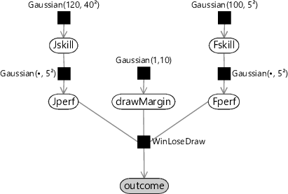
The variable Jwins is replaced by outcome which is a discrete variable that takes one of the values JillWins, Draw, or FredWins. The WinLoseDraw factor is simply a function whose value is 1 if the three values of Jperf, drawMargin, and Fperf are consistent with the value of outcome and is 0 otherwise. With this updated factor, we need to make corresponding modifications to the messages sent out from the factor node. These will not be discussed in detail here, and instead the interested reader can refer to Herbrich et al. [2007] and also an excellent blog post by Moser [2010].
In order to simplify the subsequent discussion of other extensions to the core model, we will ignore the draw modification in the remaining factor graphs in this chapter, although all subsequent models can be similarly modified to include draws if required.
What if we have more than two players in a game?

Games with more than two players require a more complex model
Suppose we now have more than two players in a game, such as in the Halo game ‘Free for All’ in which eight players simultaneously play against each other. The outcome of such a game is an ordering amongst the players involved in the game. With our model-based approach, incorporating a change such as this just involves making a suitable assumption, constructing the corresponding factor graph and then running expectation propagation again. Our new Assumptions0 3.3 can be stated as
- The order of players in the game outcome is the same as the ordering of their performance values in that game.
If there are players in the game then this assumption can be captured in a factor graph using GreaterThan factors to describe the player ordering. This is illustrated for the case of three players in Figure 3.34.
(D)(A)(B)(C)
|
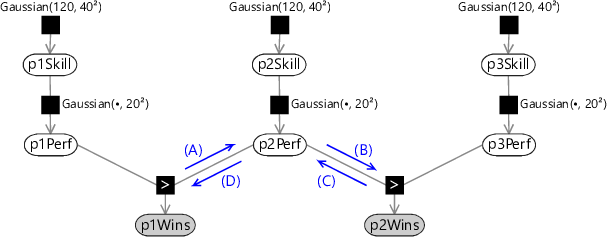
Note that we could have introduced a separate ’greater-than’ factor for each possible pair of players. For players there are such factors. However, these additional factors contain only redundant information and lead to an unnecessarily complex graph. The ordering of players can be expressed using greater than factors, provided these are chosen to connect the pairs of adjacent players in the ordering sequence. In effect, because we know the outcome of the game, we can choose a relatively simple graph which captures this.
In this optional section, we show why the use of expectation propagation, even for a tree-structured graph, can require iterative solution. If you want to focus on modelling, feel free to skip this section.
The extension to more than two players introduces an interesting effect related to our expectation propagation algorithm. We saw in section 2.2 that if our factor graph has a tree structure then belief propagation gives exact marginal distributions after a single sweep through the graph (with one message passed in each direction across every link). Similarly, if we now apply expectation propagation to the two-player graph of Figure 3.10 this again requires only a single pass in each direction. This is because the ‘context’ messages for the expectation propagation approximation are fixed. However, the situation becomes more complex when we have more than two players. The graph of Figure 3.34 has a tree structure, with no loops, and so exact belief propagation would require only a single pass. However, consider the evaluation of outgoing message (A) using expectation propagation. This requires the incoming message (D) to provide the ‘context’ for the approximation. However, message (D) depends on message (C) which itself is evaluated using expectation propagation using message (B) as context, and message (B) in turn depends on message (A). Expectation propagation therefore requires that we iterate these messages until we reach some suitable convergence criterion (in which the changes to the messages fall below some threshold). We therefore modify our message-passing schedule so that we first pass messages downwards from the skill nodes to the performance nodes (as before), then we perform multiple passes back and forth amongst the performance nodes until we achieve convergence, and then finally pass messages upwards to the skill nodes in order to evaluate posterior skill marginals.
Back in Figure 3.29 and Figure 3.30, we saw that the shift of the distributions between prior and posterior were larger in the case where the weaker player (Fred) won the game. Now we repeat the experiment, except with a third player (Steve), whose prior skill distribution is Gaussian, keeping Jill as Gaussian and Fred as Gaussian as before. We apply our multi-player TrueSkill model to a game with the outcome Jill 1st, Fred 2nd, Steve 3rd.
 Excel
Excel CSV
CSV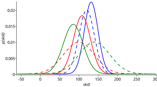
The results of this are shown in Figure 3.35. Firstly, note that since Steve was expected to be the strongest player, but in fact came last, his posterior mean has moved markedly downwards (to below the other two players). Secondly, note that the changes in the means of Jill and Fred are in the same direction as in Figure 3.29, but are more pronounced than before. This again is because the overall game result is more surprising.
Now let’s consider a different outcome with Fred and Jill swapped, so that Fred is 1st, Jill is 2nd and Steve is still in 3rd place. Figure 3.36 shows the (same) priors and the new posteriors for the three skill distributions, with this new outcome.
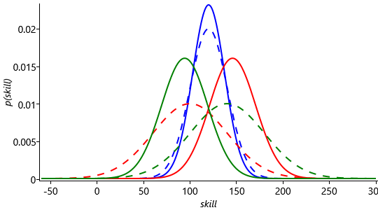
Because there is low uncertainty in Fred’s skill, his curve hardly changes given the result of the game. The fact that Fred won is strong evidence that his skill is higher than Jill or Steve’s. As a result both Jill and Steve’s skill curves move to the left of Fred’s. Because Jill beat Steve, her curve moved less than his did, so that now Steve has the lowest mean, whereas before it was the highest. What is even more interesting, if we compare Steve’s posterior skill curve in Figure 3.36 to that in Figure 3.35 is that it is even further to the left with this outcome, even though Steve came last in both cases. This is because we now have to fit Jill’s skill between that of Steve and Fred, whereas in the first outcome, Steve’s skill just had to move to the left of Fred’s. So in this multi-player game, the relative ordering of the other players has an effect on our estimate of Steve’s skill!
What if the games are played by teams?
Many of the games available on Xbox Live can be played by teams of players. For example, in Halo, another type of game is played between two teams each consisting of eight players. The outcome of the game simply says which team is the winner and which team is the loser. Our challenge is to use this information to revise the skill distributions for each of the individual players. This is an example of a credit assignment problem in which we have to work out how the credit for a victory (or blame for a defeat) should be attributed to individual players when only the outcome for the overall team is given. The solution is similar to the last two situations: we make an assumption about how the individual player skills combine to affect the game outcome, we construct a probabilistic model which encodes this assumption and then run inference to update the skill distributions. There is no need to invent new algorithms or design new heuristics.

The performance of a team depends on the skills of the individual players.
Here is one suitable assumption which we could use when modelling team games, which would replace Assumptions0 3.3:
- The performance of a team is the sum of the performances of its members, and the team with the highest performance value wins the game.
We can now build a factor graph corresponding to this assumption. For example, consider a game between two teams, each of which involves two players. The factor graph for this is shown in Figure 3.37.
|
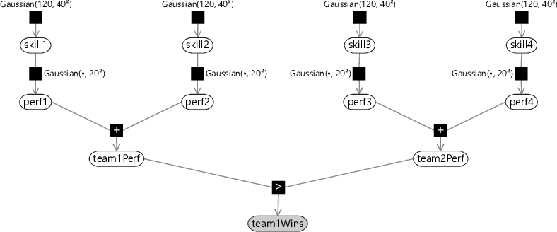
The performance of a team is determined by the performance of the players who comprise that team. Our assumption above was that the team performance is given by the sum of the performances of the individual players. This might be appropriate for collaborative team games such as Halo. However, other assumptions might be appropriate in other kinds of game. For example, in a race where only the fastest player determines the team outcome, we might make the alternative assumption
- The performance of a team is equal to the highest performance of any of its members, and the team with the highest performance value wins the game.
In this section we have discussed various modifications to the core TrueSkill model, namely the inclusion of draws, the extension to multiple players, and the extension to team games. These modifications can be combined as required, for example to allow a game between multiple teams that includes draws, by constructing the appropriate factor graph and then running expectation propagation. This highlights not only the flexibility of the model-based approach to machine learning, but also the ease with which modifications can be incorporated. As long as the model builder is able to describe the process by which the data is generated, it is usually straightforward to formulate the corresponding model. By contrast, when a solution is expressed only as an algorithm, it may be far from clear how the algorithm should be modified to account for changes in the problem specification. In the next section, we conclude our discussion of the online game matchmaking problem by a further modification to the model in which we relax the assumption that the skills of the players are fixed.
credit assignment problemThe problem of allocating a reward amongst a set of entities, such as people, all of which have contributed to the outcome.
The following exercises will help embed the concepts you have learned in this section. It may help to refer back to the text or to the concept summary below.
- Sketch out a factor graph for a model which allows draws, two-player teams and multiple teams. You will need to combine the factor graphs of Figure 3.33, Figure 3.34 and Figure 3.37. Your sketch can be quite rough – for example, you should name factors (e.g. “Gaussian”) but there is no need to provide any numbers for factor parameters.
- Extend your Infer.NET model from the previous self assessment to have three players and reproduce the results from Figure 3.35 and Figure 3.36.
- [Project idea] There is a wide variety of sports results data available on the web. Find a suitable set of data and build an appropriate model to infer the skills of the teams or players involved. Rank the teams or players by the inferred skill and decide if you think the model has inferred a good ranking. If not, diagnose why not and explore modifications to your model to address the issue.
[Herbrich et al., 2007] Herbrich, R., Minka, T., and Graepel, T. (2007). TrueSkill(TM): A Bayesian Skill Rating System. In Advances in Neural Information Processing Systems 20, pages 569–576. MIT Press.
[Moser, 2010] Moser, J. (2010). The Math behind TrueSkill.