-

Want a paper copy?
You can now buy the book!
All royalties go to the Cystic Fibrosis Trust.Spotted an error? Have comments?
Let us know!Get hands on with source code for the book.
3.5 Allowing the skills to vary
At this point we seem to have found a comprehensive solution to the problem posed at the start of the chapter. We have a probabilistic model of games between multiple teams of players including draws, in which simpler situations (two players, individuals instead of teams, games without draws) arise as special cases. However, when this system was deployed for real beta testers, it was found that its matchmaking was not always satisfactory. In particular, the skill values for some players seemed to ’get stuck’ at low values, even as the players played and improved a lot, leading to poor matchmaking.
Skill increases with practice.
To understand the reason for this we note that the assumptions encoded in our model do not allow for the skill of a player to change over time. In particular, Assumptions0 3.1 says that “each player has a skill value” – in other words, each player has a single skill value with no mention of this skill value being allowed to change. Since players’ skills do change over time, this assumption will be violated in real data. For example, as a player gains experience in playing a particular type of game, we might anticipate that their skill will improve. Conversely, an experienced player’s skill might deteriorate if they play infrequently and get out of practice.
You may think that our online learning process updates our skill distribution for a player over time and so would allow the skill to change. This is a common misconception about online learning, but it is not true. Our current model assumes that the skill of a player is a fixed, but unknown, quantity. Online learning does not represent the modelling of an evolving skill value, but rather an updating of the uncertainty in this unknown fixed-across-time skill. If a player played for a long time at a particular skill level, then our distribution over their skill would become very narrow. If the player then suddenly improved, perhaps because of some coaching, the current model would struggle to track the player’s new skill level because it would be very unlikely under the narrow skill distribution.
Reproducing the problem
To deal with players having changing skills, we will need to change the model. But first, we need to reproduce the problem, so that we can check later that we have fixed it. To do this we can create a synthetic data set. In this data set, we synthesise results of games involving a pool of one hundred players. The first player, Elliot, has an initial skill fixed at 110, and this skill value is increased in steps as shown by the red line in Figure 3.38.
 Excel
Excel CSV
CSV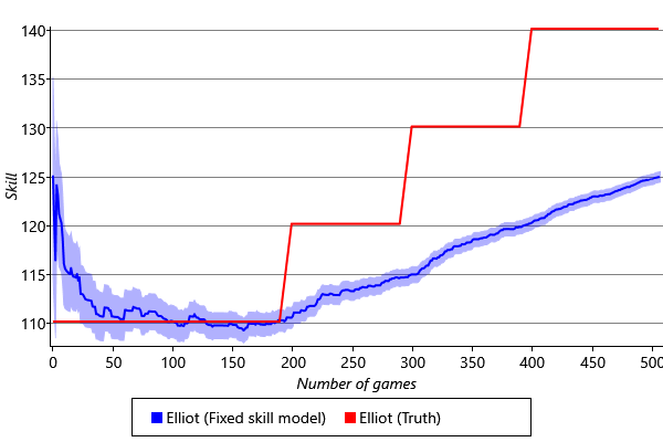
The remaining 99 players have fixed skill values which are drawn from a Gaussian with mean 125 and standard deviation 10. For each game, two players are selected at random and their performances on this game are evaluated by adding Gaussian noise to their skill values with standard deviation 5. This just corresponds to running ancestral sampling on the model in Figure 3.6 (just like we did to create a synthetic data set in section 2.5).
Given this synthetic data set, we can then run online learning using the model in Figure 3.10 in which the game outcomes are known and the skills are unknown. Figure 3.38 shows the inferred skill distribution for Elliot under this model. We see that our model cannot account for the changes in Elliot’s skill: the estimated skill mean does not match the trajectory of the true skill, and the variances of the estimates are too narrow to include the improving skill value. Due to the small variance, the update to the skill mean is small, and so the evolution of the skill mean is too slow. This is unsurprising as a key assumption of the model, namely that the skill of each player is constant, is incorrect.
To address this problem, we need to change the incorrect assumption in our model. Rather than assuming a fixed skill, we need to allow for the skill to change by a typically small amount from game to game. We can therefore replace Assumptions0 3.1 with:
- Each player has a skill value, represented by a continuous variable, given by their skill value in their previous game plus some change in skill which has a zero-mean bell-shaped distribution.
Whereas previously a player had a single skill variable, there is now a separate skill variable for each game. We assume that the skill value for a particular player in a specific game is given by the skill value from their previous game with the addition of some change in value having drawn from a zero-mean distribution. Again, we make this assumption mathematically precise by choosing this distribution to be a zero-mean Gaussian. If we denote the skill of a player in their previous game by and their skill in the current game by , then we are assuming that
where
From these two equations it follows that [Bishop, 2006]
This allows us to express our new assumption in the form of a factor graph. For example, in the case of two players who play two successive games against each other, the factor graph would be given by Figure 3.39.
|
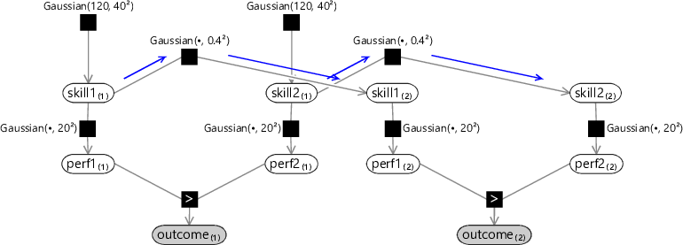
The prior distribution for skill of player 1 in the second game, denoted , is given by a Gaussian distribution whose mean, instead of being fixed, is now given by the skill of that player in the previous game, denoted by . The graph shows a ChangeVariance of 0.16 which encodes our belief that the change in skill from one game to the next should be small.
Online inference in this model can be done as follows. We run expectation propagation for the first game using a graph of the form shown in Figure 3.10, to give posterior Gaussian skill distributions for each of the players. Then we send messages through the Gaussian factors connecting the two games, as indicated in blue in Figure 3.39. The incoming messages to these factors are the skill distributions coming from the first game. The subsequent outgoing messages to the new skill variables are broadened versions of these skill distributions, because of the convolution computed for the Gaussian factor. These broadened distributions are then used as the prior skill distribution for this new game. Because we are broadening the prior in the new game, we are essentially saying that we have slightly higher uncertainty about the skill of the player. In turn, this means the new game outcome will lead to a greater change in skill, and so we will be better at tracking changes in skill. It may seem strange that we can improve the behaviour of our system by increasing the uncertainty in our skill variable, but this arises because we have modified the model to correspond more closely to reality. In the time since the last game, the player’s skill may indeed have changed and we are now correctly modelling this possibility.
We can now test out this modified model on our synthetic data set. The results are shown by the green curve in Figure 3.40.
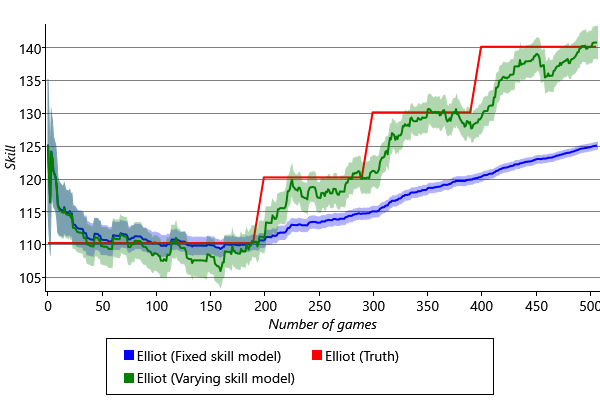
We see that the changing skill of Elliot is tracked much better when we allow for varying skills in our model – we have solved the problem of tracking time-varying skills! This model has been applied to the history of chess to work out the relative strengths of different historical chess players, even though they lived decades apart! You can read all about this work in Dangauthier et al. [2007].
The final model
Now that we have adapted the model to cope with varying skills, it meets all the requirements of the Xbox Live team. With all extensions combined, here is the full set of assumptions built into our model:
- Each player has a skill value, represented by a continuous variable, given by their skill value in their previous game plus some change in skill which has a zero-mean bell-shaped distribution.
- Each player has a performance value for each game, which is independent from game to game and has an average value is equal to the skill of that player. The variation in performance, which is the same for all players, is symmetrically distributed around the mean value and is more likely to be close to the mean than to be far from the mean.
- The performance of a team is given by the sum of the performances of the players within that team.
- The order of teams in the game outcome is the same as the ordering of their performance values in that game, unless the magnitude of the difference in performance between two teams is below a threshold in which case those teams draw.
This model encompasses the variety of different game types which arise including teams and multiple players, it allows for draws and it tracks the evolution of player skills over time. As a result, when Xbox 360 launched in November 2005, it used this TrueSkill model as its online skill rating system. Since then, the skill distributions inferred by TrueSkill have been used to perform real-time matchmaking in hundreds of different Xbox games.
The role of the model is to infer the skills, while the decision on how to use those skills to perform matchmaking is a separate question. Typically this is done by selecting players for which the game outcome is most uncertain. Note that this also tends to produce matches whose outcomes are the most informative in terms of learning the skills of the players. The matchmaking process must also take account of the need to provide players with opponents within a reasonably short time, and so there is a natural trade-off between how long a player waits for a game to be set up, and the closeness in match to their opponents. One of the powerful aspects of decomposing the matchmaking problem into the two stages of skill inference and matchmaking decision is that changes to the matchmaking criteria are easy to implement and do not require any changes to the more complex modelling and inference code. As discussed in the introduction, the ability to match players against others of similar ability, and to do so quickly and accurately, is a key feature of this very successful service.
The inferred skills produced by TrueSkill are also used for a second, distinct purpose which is to construct leaderboards showing the ranking of players within a particular type of game. For this purpose, we need to define a single skill value for each player, based on the inferred Gaussian skill distribution. One possibility would be to use the mean of the distribution, but this fails to take account of the uncertainty, and could lead to a player having an artificially high (or low) position on the leader board. Instead, the displayed skill value for a player is taken to be the mean of their distribution minus three times the standard deviation of their distribution. This is a conservative choice and implies that their actual skill is, with high probability, no lower than their displayed skill. Thus a player can make progress up the leader board both by increasing the mean of their distribution (by winning games against other players) and by reducing the uncertainty in their skill (by playing lots of games).
There are plenty of ways in which the TrueSkill model can be extended to improve its ability to model particular aspects of the game-playing process. In 2018, a number of such improvements were included in the TrueSkill 2 model [Minka et al., 2018] by making additional assumptions particularly suited to online shooters such as Gears of War and Halo. For example, the enhanced model made use of the number of kills each player made, rather than just their final ranking. It also modelled the correlation of a person’s skill in different game modes. Other improvements were made to handle situations, such as a player quitting the game mid-way through, which had previously led to inaccurate skill estimates.
We have seen how TrueSkill continually adapts to track the skill level of individual players. In the next chapter we shall see another example of a model which adapts to individual users, but in the context of a very different kind of application: helping to de-clutter your email inbox.
[Bishop, 2006] Bishop, C. M. (2006). Pattern Recognition and Machine Learning. Springer.
[Dangauthier et al., 2007] Dangauthier, P., Herbrich, R., Minka, T., and Graepel, T. (2007). Trueskill through time: Revisiting the history of chess. In Platt, J. C., Koller, D., Singer, Y., and Roweis, S. T., editors, NIPS. Curran Associates, Inc.
[Minka et al., 2018] Minka, T., Cleven, R., and Zaykov, Y. (2018). TrueSkill 2: An improved Bayesian skill rating system. Technical Report MSR-TR-2018-8, Microsoft.