-

Want a paper copy?
You can now buy the book!
All royalties go to the Cystic Fibrosis Trust.Spotted an error? Have comments?
Let us know!Get hands on with source code for the book.
8.4 K-means Clustering
K-means clustering (or simply ’k-means’) is an algorithm for dividing a set of data points into different clusters, where each cluster is defined by the mean of the points in the cluster. Data points are assigned to the cluster with the closest mean. K-means clustering is a popular method for data analysis when the goal is to identify underlying structure in a data set. The hope is that the resulting clusters will align with some underlying structure of interest. For example, suppose we have a medical data set where each data point consists of a set of relevant measurements for a person. The hope would then be that k-means clustering would result in clusters that identify useful sub-populations of people – for example, groups of people who may respond differently to treatment. K-means clustering has been around for a while – it was named ‘k-means’ in 1967 by James MacQueen [MacQueen, 1967], but the algorithm itself was developed ten years earlier by Stuart Lloyd in Bell Labs [Lloyd, 1957].
We have seen an example of doing clustering before – in section 6.5, we used a carefully constructed model to cluster children into different sensitization classes. In doing so, we made a number of assumptions about how the children should be clustered together, to ensure that the resulting sensitization classes made sense. Had we made different assumptions, the children could have been partitioned into very different clusters. Put simply, the clusters that you get out of a clustering method depend strongly on the assumptions underlying that method. This is such an important point, and one so often ignored, that it is worth repeating:
So when performing any kind of clustering, it is crucially important to understand what assumptions are being made. In this section, we will explore the assumptions underlying k-means clustering. These assumptions will allow us to understand whether clusters found using k-means will correspond well to the underlying structure of a particular data set, or not.
The k-means algorithm
The standard k-means algorithm involves alternating between two steps:
- Update assignments: given the cluster means, assign each point to the cluster with the closest mean;
- Update means: given the assignment of points to clusters, set each cluster mean to be the mean of all points assigned to that cluster.
To start alternating between these steps, you need either an initial set of means or an initial assignment of points to clusters. One common way to get an initial set of means, is to randomly select data points to be the starting cluster means. Alternatively, to get an initial assignment of points, each point can be assigned to a randomly selected cluster. This second approach is the one we will use here.
 Excel
Excel CSV
CSV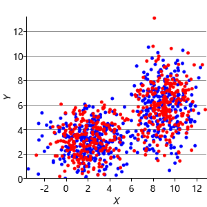
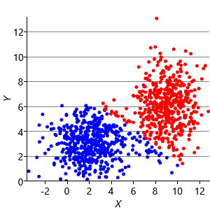
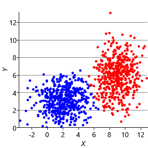

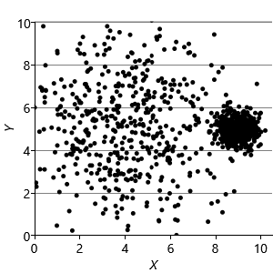
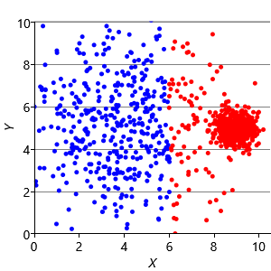
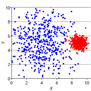
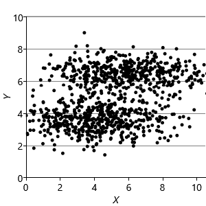
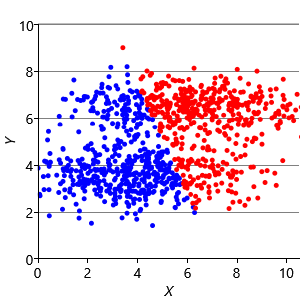
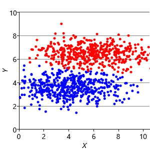
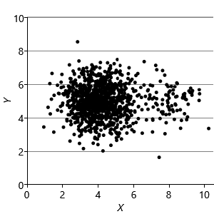
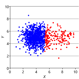
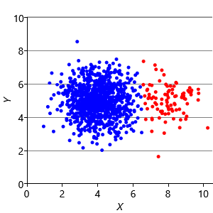
Figure 8.10a shows some an example set of data points, where the points have been randomly assigned to one of two clusters (red and blue). Given this initial assignment, the first cluster centre was set to be the mean of all blue points, and the second cluster centre to be the mean of all red points. Each data point was then assigned to the cluster with the closest centre, giving the result in Figure 8.10b. Already you can see that the colours are reasonably well aligned with the underlying clusters in the data. A further iteration gives Figure 8.10c where one data cluster is now almost entirely blue and the other almost entirely red. One more iteration causes a single data point to change colour, as shown in Figure 8.10d. Further iterations have no effect, since the assignment of points to clusters does not change.
In this example, the clusters given by k-means have done a good job at identifying the underlying structure of the data set. But will this always be the case? To answer this question, we need to express this algorithm as a model, so that we can uncover and analyse the assumptions made by the k-means algorithm.
A model for k-means
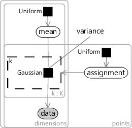
A model for the k-means algorithm needs to have variables for:
- the data, inside plates for the number of data points and for the number of dimensions;
- the mean for each cluster, inside plates for the number of clusters () and for the number of dimensions;
- the assignment for each data point, inside a plate across the data points.
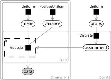
Since we don’t know anything about the mean ahead of time, the prior must be uniform across all real values. Similarly, since we don’t know anything about each assignment, the prior must be uniform across the clusters. The assignment controls which of the means the corresponding data point comes from – so we use it to turn on a gate connecting the th mean to the observed data.
The trickiest part is how to choose the factor connecting the assigned mean to each data point. To get the same result as k-means, we need a factor which gives higher probability to data points closer in distance to the cluster mean. A Gaussian factor achieves this, so long as the variance is kept fixed for all dimensions and for all clusters. Putting all this together gives the model in Figure 8.11. This factor graph is a form of a well-known model called a mixture of Gaussians.
|
To be exactly equivalent to k-means, we need the message from the gates to the assignment variable to be a point mass (‘hard’ assignment). Applying a probabilistic inference method such as expectation propagation results in a message which is a distribution over the clusters (‘soft’ assignment). Although soft assignment is generally preferable in practice, hard assignment can be achieved by setting the variance of the Gaussian factor to be extremely small. This causes the message to assignment to collapse to a point mass. Alternatively, we can just re-define the inference algorithm so that the message to assignment is defined to be a point mass at the most probable value under the distribution message. Either approach will give results identical to that of the k-means algorithm
Some hidden assumptions in k-means
The factor graph of Figure 8.11 reveals a number of assumptions hidden inside the k-means algorithm. For example, because the variance is outside the plate over the clusters, the model assumes that all the clusters have the same variance. In other words:
This assumption would not hold in a data set where the measurements vary more in one cluster than another. In a medical data set, for example, the weight of someone who has severe disease may fluctuate more than the weight of someone with milder disease and this assumption would be violated.
In Figure 8.11, the variance is also outside the plate over dimensions, which means that we assume the same amount of variability in each data dimension. Put simply:
This assumption would not be true in a data set where different measurements are in different units. In a medical data set, the units of body temperature would be different from the units of weight, and so the variation in these measurements would be on a different scale.
We’ll look at one more assumption, corresponding to the choice of prior over assignment variable. Because this prior is uniform, the model is assuming that all clusters are equally probable. This can be expressed as the assumption that:
This assumption would not hold in a data set where the underlying variable causing the clusters is not equally likely to choose any cluster. For example, in a medical data set, one underlying cluster may correspond to the most severely ill people and another to people with a milder form of the disease. If severe cases are rare compared to mild cases then this assumption would not hold.
Problems with k-means
Now that we understand the assumptions that the k-means algorithm is making, we can construct synthetic data sets to illustrate the problems these assumptions can cause. Assumptions0 8.1 is that the clusters are all the same size. So, if we make a dataset with two very different size clusters, we should expect to see k-means having problems. Figure 8.12a shows a synthetic data set with one large and one small cluster. If we run k-means clustering on this data set, we get the result shown in Figure 8.12b, where k-means has failed to discover the two clusters in the data. Instead, nearby points in the large cluster are incorrectly assigned to the small cluster, due to this incorrect assumption.
To address this problem, we can modify the factor graph to make the variance into a random variable, give it a suitable broad prior, and move it inside the plate over the clusters. With this modification, we can learn a per cluster variance and so allow clusters to be different sizes. The result of applying this model is shown in Figure 8.12c, where the two data clusters have now been correctly identified.
Assumptions0 8.2 is that clusters have the same extent in every direction. So if we make a dataset with clusters that have different extents in different directions, then we would again expect k-means to have problems. Figure 8.13a shows such a dataset, where the two clusters have been squashed vertically. Figure 8.13b shows the result of running k-means on this dataset. This result is particularly bad – k-means gives two clusters separated by a diagonal line which are not at all aligned with the actual data clusters!
We can further modify the factor graph to address the problem, by moving the variance variable inside the gate over the dimensions. This modification allows the variance to be learned per dimension, as well as per cluster. Figure 8.13c shows the result of running this modified model – now the squashed clusters in the data are correctly matched to the inferred assignments. This modification only works because the data clusters are squashed in an axis-aligned direction. To allow for the data to be squashed in any direction, we would need to change the model to learn a full covariance matrix for each cluster.
Our final assumption was that each cluster has a similar number of points (Assumptions0 8.3). Figure 8.14a shows a synthetic data set with two identically-sized clusters, but where the left-hand cluster has 90% of the data points. This imbalance makes the left-hand cluster look bigger, even though its variance is actually the same as the right-hand cluster. Because the left cluster is much more probable than the right one, points half-way between are much more likely to belong to the left cluster. If we look at the result of running k-means (Figure 8.14b), then you can see that it incorrectly assigns such points to the right-hand cluster.
We can modify our model to solve this problem by introducing a new probability vector probs, to represent the probability associated with each cluster. This modified model gives the result shown in Figure 8.14c, where the two data clusters are again nicely separated. Putting all of the above modifications together gives the factor graph of Figure 8.15. This model which makes none of these three assumptions and so has none of the associated problems.
|
Even this improved model is still making assumptions about the data which will not be true for some real data sets – for example, that the number of clusters is known or that the clusters are elliptical in shape. Further changes could be made to address these assumptions. For example, gates could be used to learn the number of clusters. We can continue this process of identifying assumptions and improving the model until it is sufficiently powerful and flexible to represent the structure of the desired data set. This ability to identify and address assumptions is the very essence of what it means to do model-based machine learning.
k-means clusteringAn algorithm for dividing a set of data points into different clusters, where each cluster is defined by the mean of the points that belong to it. Data points are assigned to the cluster with the closest mean.
Mixture of GaussiansA well-known model where each data point is generated by first selecting one of several Gaussian distributions and then sampling from that distribution.
[MacQueen, 1967] MacQueen, J. B. (1967). Some Methods for Classification and Analysis of Multivariate Observations. Proceedings of 5th Berkeley Symposium on Mathematical Statistics and Probability}, pages 281–297.
[Lloyd, 1957] Lloyd, S. P. (1957). Least square quantization in PCM. Technical report, Bell Telephone Laboratories.